Anyone using accounting measures of performance had better hope that the accounting numbers are accurate. Unfortunately, they are often not accurate, but biased. Applying EVA or any other accounting measure of performance therefore requires adjustments to the income statements and balance sheets.
For example, think of the difficulties in measuring the profitability of a pharmaceutical research program, where it typically takes 10 to 12 years to bring a new drug from discovery to final regulatory approval and the drug’s first revenues. That means 10 to 12 years of guaranteed losses, even if the managers in charge do everything right. Similar problems occur in start-up ventures, where there may be heavy capital outlays but low or negative earnings in the first years of operation. This does not imply negative NPV, so long as operating earnings and cash flows are sufficiently high later on. But EVA and ROI would be negative in the startup years, even if the project were on track to a strong positive NPV.
The problem in these cases is not with EVA or ROI, but with the accounting data. The pharmaceutical R&D program may be showing accounting losses because generally accepted accounting principles require that outlays for R&D be written off as current expenses. But from an economic point of view, those outlays are an investment, not an expense. If a proposal for a new business predicts accounting losses during a start-up period, but the proposal nevertheless shows a positive NPV, then the start-up losses are really an investment—cash outlays made to generate larger cash inflows when the business hits its stride.
1. Example: Measuring the Profitability of the Nodhead Supermarket
Supermarket chains invest heavily in building and equipping new stores. The regional manager of a chain is about to propose investing $1 million in a new store in Nodhead. Projected cash flows are
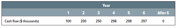
Of course, real supermarkets last more than six years. But these numbers are realistic in one important sense: It may take two or three years for a new store to build up a substantial, habitual clientele. Thus, cash flow is low for the first few years even in the best locations.
We will assume the opportunity cost of capital is 10%. The Nodhead store’s NPV at 10% is zero. It is an acceptable project, but not an unusually good one:
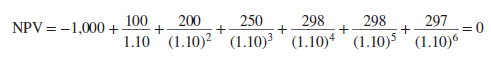
With NPV = 0, the true (internal) rate of return of this cash-flow stream is also 10%.
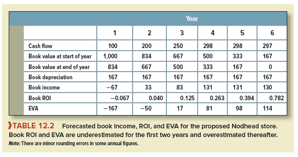
Table 12.2 shows the store’s forecasted book profitability, assuming straight-line depreciation over its six-year life. The book ROI is lower than the true return for the first two years and higher afterward.[1] EVA also starts negative for the first two years, then turns positive and grows steadily to year 6. These are typical outcomes, because accounting income is too low when a project or business is young and too high as it matures.
At this point the regional manager steps up on stage for the following soliloquy:
The Nodhead store’s a decent investment. But if we go ahead, I won’t look very good at next year’s performance review. And what if I also go ahead with the new stores in Russet, Gravenstein, and Sheepnose? Their cash-flow patterns are pretty much the same. I could actually appear to lose money next year. The stores I’ve got won’t earn enough to cover the initial losses on four new ones.
Of course, everyone knows new supermarkets lose money at first. The loss would be in the budget. My boss will understand—I think. But what about her boss? What if the board of directors starts asking pointed questions about profitability in my region? I’m under a lot of pressure to generate better earnings. Pamela Quince, the upstate manager, got a bonus for generating a positive EVA. She didn’t spend much on expansion.
The regional manager is getting conflicting signals. On the one hand, he is told to find and propose good investment projects. Good is defined by discounted cash flow. On the other hand, he is also urged to seek high book income. But the two goals conflict because book income does not measure true income. The greater the pressure for immediate book profits, the more the regional manager is tempted to forgo good investments or to favor quick payback projects over longer-lived projects, even if the latter have higher NPVs.
2. Measuring Economic Profitability
Let us think for a moment about how profitability should be measured in principle. It is easy enough to compute the true, or economic, rate of return for a common stock that is continuously traded. We just record cash receipts (dividends) for the year, add the change in price over the year, and divide by the beginning price:
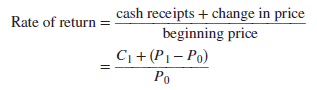
The numerator of the expression for rate of return (cash flow plus change in value) is called economic income:
Economic income = cash flow + change in present value
Any reduction in present value represents economic depreciation; any increase in present value represents negative economic depreciation. Therefore,
Economic income = cash flow – economic depreciation
The concept works for any asset. Rate of return equals cash flow plus change in value divided by starting value:
where PV0 and PV1 indicate the present values of the business at the ends of years 0 and 1.
The only hard part in measuring economic income is calculating present value. You can observe market value if the asset is actively traded, but few plants, divisions, or capital projects have shares traded in the stock market. You can observe the present market value of all the firm’s assets but not of any one of them taken separately.
Accountants rarely even attempt to measure present value. Instead they give us net book value (BV), which is original cost less depreciation computed according to some arbitrary schedule. If book depreciation and economic depreciation are different (they are rarely the same), then book earnings will not measure true earnings. (In fact, it is not clear that accountants should even try to measure true profitability. They could not do so without heavy reliance on subjective estimates of value. Perhaps they should stick to supplying objective information and leave the estimation of value to managers and investors.)
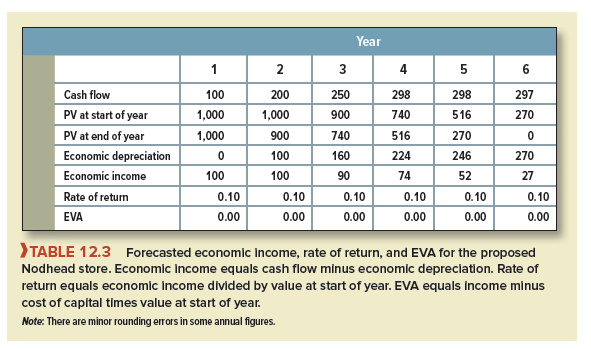
It is not hard to forecast economic income and rate of return for the Nodhead store. Table 12.3 shows the calculations. From the cash-flow forecasts we can forecast present value at the start of periods 1 to 6. Cash flow minus economic depreciation equals economic income. Rate of return equals economic income divided by start-of-period value.
Of course, these are forecasts. Actual future cash flows and values will be higher or lower. Table 12.3 shows that investors expect to earn 10% in each year of the store’s six-year life. In other words, investors expect to earn the opportunity cost of capital each year from holding this asset.
Notice that EVA calculated using present value and economic income is zero in each year of the Nodhead project’s life. For year 2, for example,
EVA = 100 – (.10 X 1,000) = 0
EVA should be zero, because the project’s true rate of return is only equal to the cost of capital. EVA will always give the right signal if, and only if, book income equals economic income and asset values are measured accurately.
3. Do the Biases Wash Out in the Long Run?
Even if the forecasts for the Nodhead store turn out to be correct, ROI and EVA will be biased if they are based on book income and book value. That might not be a serious problem if the errors wash out in the long run, when the region settles down to a steady state with an even mix of old and new stores.
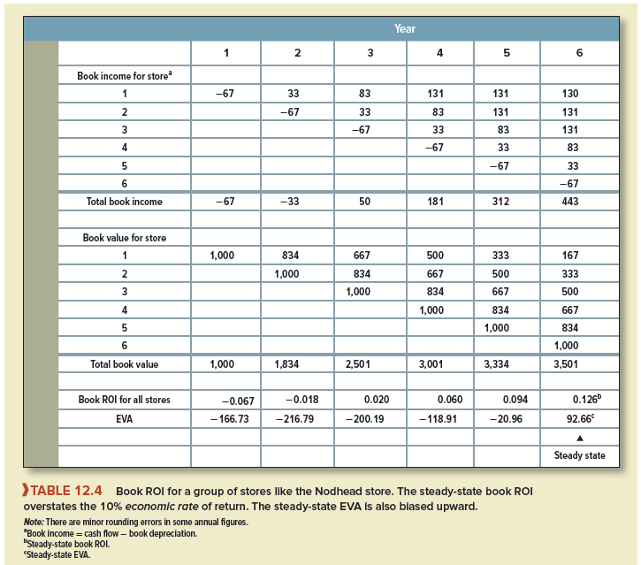
It turns out that the errors do not wash out in the steady state. Table 12.4 shows steady-state book ROIs and EVAs for the supermarket chain if it opens one store a year. For simplicity, we assume that the company starts from scratch and that each store’s cash flows are carbon copies of the Nodhead store. The true rate of return on each store is, therefore, 10% and the true EVA is zero. But as Table 12.4 demonstrates, steady-state book ROI and estimated EVA overstate the true profitability.
Thus, we still have a problem even in the long run. The extent of the error depends on how fast the business grows. We have just considered one steady state with a zero growth rate. Think of another firm with a 5% steady-state growth rate. Such a firm would invest $1,000 the first year, $1,050 the second, $1,102.50 the third, and so on. Clearly, the faster growth means more new projects relative to old ones. The greater weight given to young projects, which have low book ROIs and negative apparent EVAs, the lower the business’s apparent profitability.[2]
4. What Can We Do about Biases in Accounting Profitability Measures?
The dangers in judging profitability by accounting measures are clear from these examples. To be forewarned is to be forearmed. But we can say something beyond just “be careful.”
It is natural for firms to set a standard of profitability for plants or divisions. Ideally, that standard should be the opportunity cost of capital for investment in the plant or division. That is the whole point of EVA: to compare actual profits with the cost of capital. But if performance is measured by return on investment or EVA, then these measures need to recognize accounting biases. Ideally, the financial manager should identify and eliminate accounting biases before calculating EVA or net ROI. The managers and consultants that implement these measures work hard to adjust book income closer to economic income. For example, they may record R&D as an investment rather than an expense and construct alternative balance sheets showing R&D as an asset.
Accounting biases are notoriously hard to get rid of, however. Thus, many firms end up asking not “Did the widget division earn more than its cost of capital last year?” but “Was the widget division’s book ROI typical of a successful firm in the widget industry?” The underlying assumptions are that (1) similar accounting procedures are used by other widget manufacturers and (2) successful widget companies earn their cost of capital.
There are some simple accounting changes that could reduce biases in performance measures. Remember that the biases all stem from not using economic depreciation. Therefore, why not switch to economic depreciation? The main reason is that each asset’s present value would have to be reestimated every year. Imagine the confusion if this were attempted. You can understand why accountants set up a depreciation schedule when an investment is made and then stick to it. But why restrict the choice of depreciation schedules to the old standbys, such as straight-line? Why not specify a depreciation pattern that at least matches expected economic depreciation? For example, the Nodhead store could be depreciated according to the expected economic depreciation schedule shown in Table 12.3. This would avoid any systematic biases. It would break no law or accounting standard. This step seems so simple and effective that we are at a loss to explain why firms have not adopted it.
25 Jun 2021
23 Jun 2021
24 Jun 2021
24 Jun 2021
25 Jun 2021
24 Jun 2021