The Relationship between Risk and Return

In Chapter 7, we looked at the returns on selected investments. The least risky investment was U.S. Treasury bills. Since the return on Treasury bills is fixed, it is unaffected by what hap­pens to the market. In other words, Treasury bills have a beta of 0. We also considered a much riskier investment, the market portfolio of common stocks. This has average market risk: Its beta is 1.0.

Wise investors don’t take risks just for fun. They are playing with real money. Therefore, they require a higher return from the market portfolio than from Treasury bills. The differ­ence between the return on the market and the interest rate is termed the market risk premium. Since 1900, the market risk premium (r_m – rf) has averaged 7.7% a year.

In Figure 8.6, we have plotted the risk and expected return from Treasury bills and the market portfolio. You can see that Treasury bills have a beta of 0 and a risk premium of 0.^[1] The market portfolio has a beta of 1 and a risk premium of r_m – r. This gives us two bench­marks for an investment’s expected risk premium. But what risk premium can one look forward to when beta is not 0 or 1?

In the mid-1960s three economists—William Sharpe, John Lintner, and Jack Treynor— produced an answer to this question.^[2] Their answer is known as the capital asset pricing model, or CAPM. The model’s message is both startling and simple. In a competitive market, the expected risk premium varies in direct proportion to beta. This means that in Figure 8.6 all investments must plot along the sloping line, known as the security market line. The expected risk premium on an investment with a beta of .5 is, therefore, half the expected risk premium on the market; the expected risk premium on an investment with a beta of 2 is twice the expected risk premium on the market. We can write this relationship as

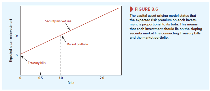
Expected risk premium on stock = beta X expected risk premium on market

r − ​r f  = β ( r m  − ​r f )

1. Some Estimates of Expected Returns

Before we tell you where the formula comes from, let us use it to figure out what returns investors are looking for from particular stocks. To do this, we need three numbers: p, rf, and r_m – rf. We gave you estimates of the betas of 10 stocks in Table 7.5. We will suppose that the interest rate on Treasury bills is about 2%.

Table 8.2 puts these numbers together to give an estimate of the expected return on each stock. The stock with the highest beta in our sample is U.S. Steel. Our estimate of the expected return from U.S. Steel is 22.3%. The stock with the lowest beta is Newmont. Our estimate of its expected return is just 2.7%. Notice that these expected returns are not the same as the hypothetical forecasts of return that we assumed in Table 8.1 to gener­ate the efficient frontier. They are the returns that investors can expect if the stocks are fairly priced.

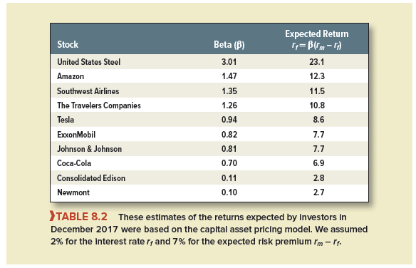
You can also use the capital asset pricing model to find the discount rate for a new capital investment. For example, suppose that you are analyzing a proposal by Coca-Cola to expand its business. At what rate should you discount the forecasted cash flows? According to Table 8.2, investors are looking for a return of 6.9% from businesses with the risk of Coca-Cola. So the cost of capital for a further investment in the same business is 6.9%.

In practice, choosing a discount rate is seldom so easy. (After all, you can’t expect to be paid a fat salary just for plugging numbers into a formula.) For example, you must learn how to adjust the expected return to remove the extra risk caused by company borrowing. Also you need to consider the difference between short- and long-term interest rates. As we write this in February 2018, the interest rate on Treasury bills is well below long-term rates. It is possible that investors were content with the prospect of quite modest equity returns in the short run, but they almost certainly required higher long-run returns. If that is so, a cost of capital based on short-term rates may be inappropriate for long-term capital investments. In Table 8.2, we largely sidestepped the issue by arbitrarily assuming an interest rate of 2%. We will return later to some of these refinements.

2. Review of the Capital Asset Pricing Model

Let us review the basic principles of portfolio selection:

1. Investors like high expected return and low standard deviation. Common stock portfolios that offer the highest expected return for a given standard deviation are known as efficient portfolios.
2. If the investor can lend or borrow at the risk-free rate of interest, one efficient portfolio is better than all the others: the portfolio that offers the highest ratio of risk premium to standard deviation (i.e., portfolio S in Figure 8.5). A risk-averse investor will put part of his money in this efficient portfolio and part in the risk-free asset. A risk-tolerant investor may put all her money in this portfolio or she may borrow and put in even more.

3. The composition of this best efficient portfolio depends on the investor’s assessments of expected returns, standard deviations, and correlations. But suppose everybody has the same information and the same assessments. If no one has any superior information, each investor should hold the same portfolio as everybody else; in other words, everyone should hold the market portfolio.

Now let us go back to the risk of individual stocks:

4. Do not look at the risk of a stock in isolation but at its contribution to portfolio risk. This contribution depends on the stock’s sensitivity to changes in the value of the portfolio.

5. A stock’s sensitivity to changes in the value of the market portfolio is known as Beta, therefore, measures the marginal contribution of a stock to the risk of the market portfolio.

Now if everyone holds the market portfolio, and if beta measures each security’s contribution to the risk of the market portfolio, then it is no surprise that the risk premium demanded by investors is proportional to beta. That is the message of the CAPM.

3. What If a Stock Did Not Lie on the Security Market Line?

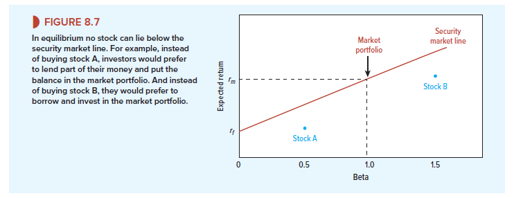
Imagine that you encounter stock A in Figure 8.7. Would you buy it? We hope not^[5]—if you want an investment with a beta of .5, you could get a higher expected return by investing half your money in Treasury bills and half in the market portfolio. If everybody shares your view of the stock’s prospects, the price of A will have to fall until the expected return matches what you could get elsewhere.

What about stock B in Figure 8.7? Would you be tempted by its high return? You wouldn’t if you were smart. You could get a higher expected return for the same beta by borrowing 50 cents for every dollar of your own money and investing in the market portfolio. Again, if everybody agrees with your assessment, the price of stock B cannot hold. It will have to fall until the expected return on B is equal to the expected return on the combination of borrowing and investment in the market portfolio.^[6]

We have made our point. An investor can always obtain an expected risk premium of P(r_m – ^rf) by holding a mixture of the market portfolio and a risk-free loan. So in well­functioning markets nobody will hold a stock that offers an expected risk premium of less than p(r_m – rf). But what about the other possibility? Are there stocks that offer a higher expected risk premium? In other words, are there any that lie above the security market line in Figure 8.7? If we take all stocks together, we have the market portfolio. Therefore, we know that stocks on average lie on the line. Since none lies below the line, then there also can’t be any that lie above the line. Thus each and every stock must lie on the security market line and offer an expected risk premium of

r − ​r f  = β ( r m  − ​r f )

Source:  Brealey Richard A., Myers Stewart C., Allen Franklin (2020), Principles of Corporate Finance, McGraw-Hill Education; 13th edition.