Population Mean: s Unknown

When developing an interval estimate of a population mean we usually do not have a good estimate of the population standard deviation either. In these cases, we must use the same sample to estimate both m and s. This situation represents the s unknown case. When 5 is used to estimate s, the margin of error and the interval estimate for the population mean are based on a probability distribution known as the t distribution. Although the mathem­atical development of the t distribution is based on the assumption of a normal distribution for the population we are sampling from, research shows that the t distribution can be successfully applied in many situations where the population deviates significantly from normal. Later in this section we provide guidelines for using the t distribution if the popu­lation is not normally distributed.

The t distribution is a family of similar probability distributions, with a specific t distri­bution depending on a parameter known as the degrees of freedom. The t distribution with one degree of freedom is unique, as is the t distribution with two degrees of freedom, with three degrees of freedom, and so on. As the number of degrees of freedom increases, the difference between the t distribution and the standard normal distribution becomes smaller and smaller. Figure 8.4 shows t distributions with 10 and 20 degrees of freedom and their relationship to the standard normal probability distribution. Note that a t distribution with more degrees of freedom exhibits less variability and more closely resembles the standard normal distribution. Note also that the mean of the t distribution is zero.

We place a subscript on t to indicate the area in the upper tail of the t distribution. For example, just as we used z.₀₂₅ to indicate the z value providing a .025 area in the upper tail of a standard normal distribution, we will use t.₀₂₅ to indicate a .025 area in the upper tail of a t distribution. In general, we will use the notation t_a/2 to represent a t value with an area of a/2 in the upper tail of the t distribution. See Figure 8.5.

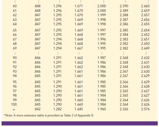
Table 2 in Appendix B contains a table for the t distribution. A portion of this table is shown in Table 8.2. Each row in the table corresponds to a separate t distribution with the degrees of freedom shown. For example, for a t distribution with 9 degrees of freedom, t.₀₂₅ = 2.262. Similarly, for a t distribution with 60 degrees of freedom, t.₀₂₅ = 2.000.

As the degrees of freedom continue to increase, t.₀₂₅ approaches z.₀₂₅ = 1 96. In fact, the standard normal distribution z values can be found in the infinite degrees of freedom row (labeled “) of the t distribution table. If the degrees of freedom exceed 100, the infinite degrees of freedom row can be used to approximate the actual t value; in other words, for more than 100 degrees of freedom, the standard normal z value provides a good approx­imation to the t value.

1. Margin of Error and the Interval Estimate

In Section 8.1 we showed that an interval estimate of a population mean for the s known case is

To compute an interval estimate of μ for the s unknown case, the sample standard devi­ation i is used to estimate s, and z_a/2 is replaced by the t distribution value t_a/2. The margin of error is then given by t_a/2 s/√n. With this margin of error, the general expression for an interval estimate of a population mean when s is unknown follows.

The reason the number of degrees of freedom associated with the t value in expression (8.2) is n -1 concerns the use of s as an estimate of the population standard deviation σ. The expression for the sample standard deviation is

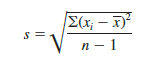
Degrees of freedom refer to the number of independent pieces of information that go into the computation of ∑(x_i – x)². The n pieces of information involved in computing ∑(x_; – x)² are as follows: x₁ – x, x₂ – x, . . . , x_n – x. In Section 3.2 we indicated that ∑(x_; – x) = 0 for any data set. Thus, only n – 1 of the x_t – x values are independent; that is, if we know n – 1 of the values, the remaining value can be determined exactly by using the condition that the sum of the x_t – x values must be 0. Thus, n – 1 is the number of degrees of freedom associated with ∑(x_; – x)² and hence the number of degrees of freedom for the t distribution in expression (8.2).

To illustrate the interval estimation procedure for the s unknown case, we will consider a study designed to estimate the mean credit card debt for the population of U.S. households. A sample of n = 70 households provided the credit card balances shown in Table 8.3. For this situation, no previous estimate of the population stand­ard deviation s is available. Thus, the sample data must be used to estimate both the population mean and the population standard deviation. Using the data in Table 8.3, we compute the sample mean x = $9312 and the sample standard deviation 5 = $4007. With 95% confidence and n – 1 = 69 degrees of freedom, Table 8.2 can be used to obtain the appropriate value for t.₀₂₅. We want the t value in the row with 69 degrees of freedom, and the column corresponding to .025 in the upper tail. The value shown is ^t.025 = 1.995.

We use expression (8.2) to compute an interval estimate of the population mean credit card balance.

The point estimate of the population mean is $9312, the margin of error is $955, and the 95% confidence interval is 9312 – 955 = $8357 to 9312 + 955 = $10,267. Thus, we are 95% confident that the mean credit card balance for the population of all households is between $8357 and $10,267.

The procedures used by JMP and Excel to develop confidence intervals for a popula­tion mean are described in Appendixes 8.1 and 8.2. For the household credit card balances study, the sample of 70 households provides a sample mean credit card balance of $9312, a sample standard deviation of $4007, a standard error of the mean of $479, and a 95% confidence interval of $8357 to $10,267.

2. Practical Advice

If the population follows a normal distribution, the confidence interval provided by expres­sion (8.2) is exact and can be used for any sample size. If the population does not follow a normal distribution, the confidence interval provided by expression (8.2) will be approx­imate. In this case, the quality of the approximation depends on both the distribution of the population and the sample size.

In most applications, a sample size of n > 30 is adequate when using expression (8.2) to develop an interval estimate of a population mean. However, if the population distribu­tion is highly skewed or contains outliers, most statisticians would recommend increasing the sample size to 50 or more. If the population is not normally distributed but is roughly symmetric, sample sizes as small as 15 can be expected to provide good approximate confidence intervals. With smaller sample sizes, expression (8.2) should only be used if the analyst believes, or is willing to assume, that the population distribution is at least approxi­mately normal.

3. Using a Small Sample

In the following example we develop an interval estimate for a population mean when the sample size is small. As we already noted, an understanding of the distribution of the population becomes a factor in deciding whether the interval estimation procedure provides acceptable results.

Scheer Industries is considering a new computer-assisted program to train maintenance employees to do machine repairs. In order to fully evaluate the program, the director of manufacturing requested an estimate of the population mean time required for maintenance employees to complete the computer-assisted training.

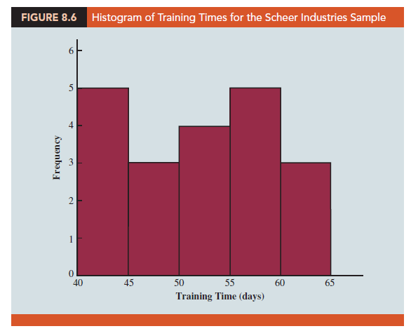
A sample of 20 employees is selected, with each employee in the sample completing the training program. Data on the training time in days for the 20 employees are shown in Table 8.4. A histogram of the sample data appears in Figure 8.6. What can we say about the distribution of the population based on this histogram? First, the sample data do not support the conclusion that the distribution of the population is normal, yet we do not see any evidence of skewness or outliers. Therefore, using the guidelines in the previous sub­section, we conclude that an interval estimate based on the t distribution appears acceptable for the sample of 20 employees.

We continue by computing the sample mean and sample standard deviation as follows.

For a 95% confidence interval, we use Table 2 of Appendix B and n – 1 = 19 degrees of freedom to obtain t.₀₂₅ = 2.093. Expression (8.2) provides the interval estimate of the population mean.

The point estimate of the population mean is 51.5 days. The margin of error is 3.2 days and the 95% confidence interval is 51.5 – 3.2 = 48.3 days to 51.5 + 3.2 = 54.7 days.

Using a histogram of the sample data to learn about the distribution of a population is not always conclusive, but in many cases it provides the only information available. The histogram, along with judgment on the part of the analyst, can often be used to decide whether expression (8.2) can be used to develop the interval estimate.

4. Summary of Interval Estimation Procedures

We provided two approaches to developing an interval estimate of a population mean. For the s known case, s and the standard normal distribution are used in expression (8.1) to compute the margin of error and to develop the interval estimate. For the s unknown case, the sample standard deviation s and the t distribution are used in expression (8.2) to com­pute the margin of error and to develop the interval estimate.

A summary of the interval estimation procedures for the two cases is shown in Figure 8.7. In most applications, a sample size of n ≥ 30 is adequate. If the population has a normal or approximately normal distribution, however, smaller sample sizes may be used. For the s unknown case a sample size of n ≥ 50 is recommended if the population distribution is believed to be highly skewed or has outliers.

Source:  Anderson David R., Sweeney Dennis J., Williams Thomas A. (2019), Statistics for Business & Economics, Cengage Learning; 14th edition.