The Binomial Method for Valuing Options

The essential trick in pricing any option is to set up a package of investments in the stock and the loan that will exactly replicate the payoffs from the option. If we can price the stock and the loan, then we can also price the option. Equivalently, we can pretend that investors are risk-neutral, calculate the expected payoff on the option in this fictitious risk-neutral world, and discount by the rate of interest to find the option’s present value.

These concepts are completely general, but the example in the last section used a simpli­fied version of what is known as the binomial method. The method starts by reducing the possible changes in the next period’s stock price to two, an “up” move and a “down” move. This assumption that there are just two possible prices for Amazon stock at the end of six months is clearly fanciful.

We could make the Amazon problem a trifle more realistic by assuming that there are two possible price changes in each three-month period. This would give a wider variety of six- month prices. And there is no reason to stop at three-month periods. We could go on to take shorter and shorter intervals, with each interval showing two possible changes in Amazon’s stock price and giving an even wider selection of six-month prices.

We illustrate this in Figure 21.1. The top diagram shows our starting assumption: just two possible prices at the end of six months. Moving down, you can see what happens when there are two possible price changes every three months. This gives three possible stock prices when the option matures. In Figure 21.1c, we have gone on to divide the six-month period into 26 weekly periods, in each of which the price can make one of two small moves. The distribution of prices at the end of six months is now looking much more realistic.

We could continue in this way to chop the period into shorter and shorter intervals, until eventually we would reach a situation in which the stock price is changing continuously and there is a continuum of possible future stock prices. We demonstrate first with our simple two-step case in Figure 21.1b. Then we work up to the situation where the stock price is changing continuously. Don’t panic; that won’t be as bad as it sounds.

1. Example: The Two-Step Binomial Method

Dividing the period into shorter intervals doesn’t alter the basic approach for valuing a call option. We can still find at each point a levered investment in the stock that gives exactly the same payoffs as the option. The value of the option must therefore be equal to the value of this replicating portfolio. Alternatively, we can pretend that investors are risk-neutral and expect to earn the interest rate on all their investments. We then calculate at each point the expected future value of the option and discount it at the risk-free interest rate. Both methods give the same answer.

If we use the replicating-portfolio method, we must recalculate the investment in the stock at each point, using the formula for the option delta:

Recalculating the option delta is not difficult, but it can become a bit of a chore. It is simpler in this case to use the risk-neutral method, and that is what we will do.

Figure 21.2 is taken from Figure 21.1 and shows the possible prices of Amazon stock, assuming that in each three-month period the price will either rise by 13.76% or fall by 12.10%.⁷ We show in parentheses the possible values at maturity of a six-month call option with an exercise price of $900. For example, if Amazon’s stock price turns out to be $695.45 in month 6, the call option will be worthless; at the other extreme, if the stock value is $1,164.72, the call will be worth $1,164.72 – $900 = $264.72. We haven’t worked out yet what the option will be worth before maturity, so we will just put question marks there for now.

We continue to assume an interest rate of .5% for 6 months, which is equivalent to about .25% a quarter. We now ask: If investors demand a return of .25% a quarter, what is the prob­ability (p) at each stage that the stock price will rise? The answer is given by our simple formula:

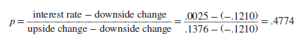
We can check that if there is a 47.74% chance of a rise of 13.76% and a 52.26% chance of a fall of 12.10%, then the expected return must be equal to the .25% risk-free rate:

(.4774 x 13.76) + (.5226 x -12.10) = .25%

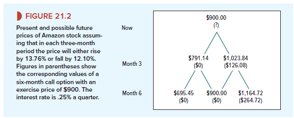
Option Value in Month 3 Now we can find the possible option values in month 3. Suppose that by the end of three months, the stock price has risen to $1,023.84. In that case, investors know that when the option finally matures in month 6, the option value will be either $0 or $264.72. We can therefore use our risk-neutral probabilities to calculate the expected option value at month 6:

Expected value of call in month 6 = (probability of rise X 264.72) + (probability of fall X 0)

                                    = (.4774 X 264.72) + (.5226 X 0) = $126.39

And the value in month 3 is 126.39/1.0025 = $126.08.

What if the stock price falls to $791.14 by month 3? In that case the option is bound to be worthless at maturity. Its expected value is zero, and its value at month 3 is also zero.

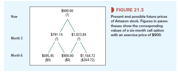
Option Value Today We can now get rid of two of the question marks in Figure 21.2. Figure 21.3 shows that if the stock price in month 3 is $1,023.84, the option value is $126.08, and if the stock price is $791.14, the option value is zero. It only remains to work back to the option value today.

There is a 47.74% chance that the option will be worth $126.08 and a 52.26% chance that it will be valueless. So the expected value in month 3 is

(.4774 X 126.08) + (.5626 X 0) = $60.19

And the value today is 60.19/1.0025 = $60.05.

2. The General Binomial Method

Moving to two steps when valuing the Amazon call probably added extra realism. But there is no reason to stop there. We could go on, as in Figure 21.1, to chop the period into smaller and smaller intervals. We could still use the binomial method to work back from the final date to the present. Of course, it would be tedious to do the calculations by hand but simple to do so with a computer.

Since a stock can usually take on an almost limitless number of future values, the binomial method gives a more realistic and accurate measure of the option’s value if we work with a large number of subperiods. But that raises an important question. How do we pick sen­sible figures for the up and down changes in value? For example, why did we pick figures of +13.76% and -12.1% when we revalued Amazon’s option with two subperiods? Fortunately,

there is a neat little formula that relates the up and down changes to the standard deviation of stock returns:

where

e = base for natural logarithms = 2.718

σ = standard deviation of (continuously compounded) stock returns

h = interval as fraction of a year

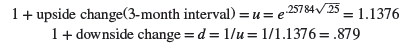
When we said that Amazon’s stock price could either rise by 20% or fall by 16.667% over six months (h = .5), our figures were consistent with a figure of 25.784% for the standard devia­tion of annual returns:^[1]

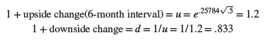
To work out the equivalent upside and downside changes when we divide the period into two three-month intervals (h = .25), we use the same formula:

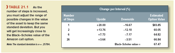
The center columns in Table 21.1 show the equivalent up and down moves in the value of the firm if we chop the period into six monthly or 26 weekly periods, and the final column shows the effect on the estimated option value. (We explain the Black-Scholes value shortly.)

3. The Binomial Method and Decision Trees

Calculating option values by the binomial method is basically a process of solving decision trees. You start at some future date and work back through the tree to the present. Eventually, the possible cash flows generated by future events and actions are folded back to a present value.

Is the binomial method merely another application of decision trees, a tool of analysis that you learned about in Chapter 10? The answer is no, for at least two reasons. First, option pric­ing theory is absolutely essential for discounting within decision trees. Discounting expected cash flows doesn’t work within decision trees for the same reason that it doesn’t work for puts and calls. As we pointed out in Section 21-1, there is no single, constant discount rate for options because the risk of the option changes as time and the price of the underlying asset change. There is no single discount rate inside a decision tree because, if the tree contains meaningful future decisions, it also contains options. The market value of the future cash flows described by the decision tree has to be calculated by option pricing methods.

Second, option theory gives a simple, powerful framework for describing complex deci­sion trees. For example, suppose that you have the option to abandon an investment. The complete decision tree would overflow the largest classroom whiteboard. But now that you know about options, the opportunity to abandon can be summarized as “an American put.” Of course, not all real problems have such easy option analogies, but we can often approximate complex decision trees by some simple package of assets and options. A custom decision tree may get closer to reality, but the time and expense may not be worth it. Most men buy their suits off the rack even though a custom-made Armani suit would fit better and look nicer.

Source:  Brealey Richard A., Myers Stewart C., Allen Franklin (2020), Principles of Corporate Finance, McGraw-Hill Education; 13th edition.