Many projects require a heavy initial outlay on new production facilities. But often the largest investments involve the acquisition of intangible assets. For example, U.S. banks invest huge sums annually in new information technology (IT) projects. Much of this expenditure goes to intangibles such as system design, programming, testing, and training. Think also of the huge expenditure by pharmaceutical companies on research and development (R&D). Merck, one of
the largest pharmaceutical companies, spends more than $7 billion a year on R&D. The R&D cost of bringing one new prescription drug to market has been estimated at more than $2 billion.
Expenditures on intangible assets such as IT and R&D are investments just like expenditures on new plant and equipment. In each case, the company is spending money today in the expectation that it will generate a stream of future profits. Ideally, firms should apply the same criteria to all capital investments, regardless of whether they involve a tangible or intangible asset.
We have seen that an investment in any asset creates wealth if the discounted value of the future cash flows exceeds the up-front cost. Up to this point, however, we have glossed over the problem of what to discount. When you are faced with this problem, you should stick to five general rules:
- Discount cash flows, not profits.
- Discount incremental cash flows.
- Treat inflation consistently.
- Separate investment and financing decisions.
- Forecast and deduct taxes.
We discuss each of these rules in turn.
1. Rule 1: Discount Cash Flows, Not Profits
The first and most important point: Net present value depends on the expected future cash flow. Cash flow is simply the difference between cash received and cash paid out. Many people nevertheless confuse cash flow with accounting income. Accounting income is intended to show how well the company is performing. Therefore, accountants start with “dollars in” and “dollars out,” but to obtain accounting income, they adjust these inputs in two principal ways.
Capital Expenses When calculating expenditures, the accountant deducts current expenses but does not deduct capital expenses. There is a good reason for this. If the firm lays out a large amount of money on a big capital project, you do not conclude that the firm is performing poorly, even though a lot of cash is going out the door. Therefore, instead of deducting capital expenditure as it occurs, the accountant depreciates the outlay over several years.
That makes sense when judging firm performance, but it will get you into trouble when working out net present value. For example, suppose that you are analyzing an investment proposal. It costs $2,000 and is expected to provide a cash flow of $1,500 in the first year and $500 in the second. If the accountant depreciates the capital expenditure straight line over the two years, accounting income is $500 in year 1 and -$500 in year 2:
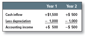
Suppose you were given this forecast income and naively discounted it at 10%. NPV would appear positive:
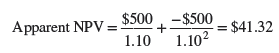
This has to be nonsense. The project is obviously a loser. You are laying out $2,000 today and simply getting it back later. At any positive discount rate the project has a negative NPV.
The message is clear: When calculating NPV, state capital expenditures when they occur, not later when they show up as depreciation. To go from accounting income to cash flow, you need to add back depreciation (which is not a cash outflow) and subtract capital expenditure (which is a cash outflow).
Working Capital When measuring income, accountants try to show profit as it is earned, rather than when the company and its customers get around to paying their bills.
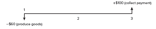
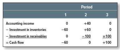
For example, consider a company that spends $60 to produce goods in period 1. It sells these goods in period 2 for $100, but its customers do not pay their bills until period 3. The following diagram shows the firm’s cash flows. In period 1 there is a cash outflow of $60. Then, when customers pay their bills in period 3, there is an inflow of $100.
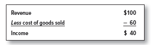
It would be misleading to say that the firm was running at a loss in period 1 (when cash flow was negative) or that it was extremely profitable in period 3 (when cash flow was positive). Therefore, the accountant looks at when the sale was made (period 2 in our example) and gathers together all the revenues and expenses associated with that sale. In the case of our company, the accountant would show for period 2.
Of course, the accountant cannot ignore the actual timing of the cash expenditures and payments. So the $60 cash outlay in the first period will be treated not as an expense but as an investment in inventories. Subsequently, in period 2, when the goods are taken out of inventory and sold, the accountant shows a $60 reduction in inventories.
The accountant also does not ignore the fact that the firm has to wait to collect on its bills. When the sale is made in period 2, the accountant will record accounts receivable of $100 to show that the company’s customers owe $100 in unpaid bills. Later, when the customers pay those bills in period 3, accounts receivable are reduced by that $100.
To go from the figure for income to the actual cash flows, you need to add back these changes in inventories and receivables:
Net working capital (often referred to simply as working capital) is the difference between a company’s short-term assets and liabilities. Accounts receivable and inventories of raw materials, work in progress, and finished goods are the principal short-term assets. The principal short-term liabilities are accounts payable (bills that you have not paid) and taxes that have been incurred but not yet paid.[1]
Most projects entail an investment in working capital. Each period’s change in working capital should be recognized in your cash-flow forecasts.[2] By the same token, when the project comes to an end, you can usually recover some of the investment. This results in a cash inflow. (In our simple example the company made an investment in working capital of $60 in period 1 and $40 in period 2. It made a disinvestment of $100 in period 3, when the customers paid their bills.)
Working capital is a common source of confusion in capital investment calculations. Here are the most common mistakes:
- Forgetting about working capital entirely. We hope that you do not fall into that trap.
- Forgetting that working capital may change during the life of the project. Imagine that you sell $100,000 of goods a year and customers pay on average six months late. You therefore have $50,000 of unpaid bills. Now you increase prices by 10%, so revenues increase to $110,000. If customers continue to pay six months late, unpaid bills increase to $55,000, and so you need to make an additional investment in working capital of $5,000.
- Forgetting that working capital is recovered at the end of the project. When the project comes to an end, inventories are run down, any unpaid bills are (you hope) paid off, and you recover your investment in working capital. This generates a cash
2. Rule 2: Discount Incremental Cash Flows
The value of a project depends on all the additional cash flows that follow from project acceptance. Here are some things to watch for when you are deciding which cash flows to include.
Include All Incidental Effects It is important to consider a project’s effects on the remainder of the firm’s business. For example, suppose Sony proposes to launch PlayStation X, a new version of its videogame console. Demand for the new product will almost certainly cut into sales of Sony’s existing consoles. This incidental effect needs to be factored into the incremental cash flows. Of course, Sony may reason that it needs to go ahead with the new product because its existing product line is likely to come under increasing threat from competitors. So, even if it decides not to produce the new PlayStation, there is no guarantee that sales of the existing consoles will continue at their present level. Sooner or later, they will decline.
Sometimes a new project will help the firm’s existing business. Suppose that you are the financial manager of an airline that is considering opening a new short-haul route from Harrisburg, Pennsylvania, to Chicago’s O’Hare Airport. When considered in isolation, the new route may have a negative NPV. But once you allow for the additional business that the new route brings to your other traffic out of O’Hare, it may be a very worthwhile investment.
Do Not Confuse Average with Incremental Payoffs Most managers naturally hesitate to throw good money after bad. For example, they are reluctant to invest more money in a losing division. But occasionally you will encounter turnaround opportunities in which the incremental NPV from investing in a loser is strongly positive.
Conversely, it does not always make sense to throw good money after good. A division with an outstanding past profitability record may have run out of good opportunities. You would not pay a large sum for a 20-year-old horse, sentiment aside, regardless of how many races that horse had won or how many champions it had sired.
Here is another example illustrating the difference between average and incremental returns: Suppose that a railroad bridge is in urgent need of repair. With the bridge the railroad can continue to operate; without the bridge it can’t. In this case, the payoff from the repair work consists of all the benefits of operating the railroad. The incremental NPV of such an investment may be enormous. Of course, these benefits should be net of all other costs and all subsequent repairs; otherwise, the company may be misled into rebuilding an unprofitable railroad piece by piece.
Forecast Product Sales but also Recognize After-Sales Cash Flows Financial managers should forecast all incremental cash flows generated by an investment. Sometimes these incremental cash flows last for decades. When GE commits to the design and production of a new jet engine, the cash inflows come first from the sale of engines and then from service and spare parts. A jet engine will be in use for 30 years. Over that period revenues from service and spare parts will be roughly seven times the engine’s purchase price.
Many other manufacturing companies depend on the revenues that come after their products are sold. For example, the consulting firm Accenture estimates that services and parts typically account for about 25% of revenues and 50% of profits for auto companies.3
Include Opportunity Costs The cost of a resource may be relevant to the investment decision even when no cash changes hands. For example, suppose a new manufacturing operation uses land that could otherwise be sold for $100,000. This resource is not free: It has an opportunity cost, which is the cash it could generate for the company if the project were rejected and the resource were sold or put to some other productive use.
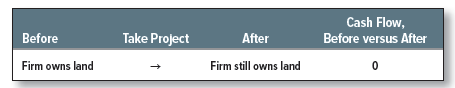
This example prompts us to warn you against judging projects on the basis of “before versus after.” The proper comparison is “with or without.” A manager comparing before versus after might not assign any value to the land because the firm owns it both before and after:
The proper comparison, with or without, is as follows:
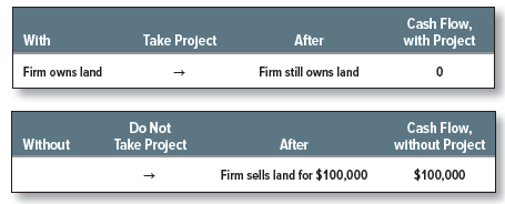
Comparing the two possible “afters,” we see that the firm gives up $100,000 by undertaking the project. This reasoning still holds if the land will not be sold but is worth $100,000 to the firm in some other use.
Sometimes opportunity costs may be very difficult to estimate; however, where the resource can be freely traded, its opportunity cost is simply equal to the market price. Consider a widely used aircraft such as the Boeing 737. Secondhand 737s are regularly traded, and their prices are quoted on the web. So, if an airline needs to know the opportunity cost of continuing to use one of its 737s, it just needs to look up the market price of a similar plane. The opportunity cost of using the plane is equal to the cost of buying an equivalent aircraft to replace it.
Forget Sunk Costs Sunk costs are like spilled milk: They are past and irreversible outflows. Because sunk costs are bygones, they cannot be affected by the decision to accept or reject the project, and so they should be ignored.
Take the case of the James Webb Space Telescope. It was originally supposed to launch in 2011 and cost $1.6 billion. But the project became progressively more expensive and further behind schedule. Latest estimates put the cost at $8.8 billion and a launch date of 2019. When Congress debated whether to cancel the program, supporters of the project argued that it would be foolish to abandon a project on which so much had already been spent. Others countered that it would be even more foolish to continue with a project that had proved so costly. Both groups were guilty of the sunk-cost fallacy; the money that had already been spent by NASA was irrecoverable and, therefore, irrelevant to the decision to terminate the project.
Beware of Allocated Overhead Costs We have already mentioned that the accountant’s objective is not always the same as the investment analyst’s. A case in point is the allocation of overhead costs. Overheads include such items as supervisory salaries, rent, heat, and light. These overheads may not be related to any particular project, but they have to be paid for somehow. Therefore, when the accountant assigns costs to the firm’s projects, a charge for overhead is usually made. Now our principle of incremental cash flows says that in investment appraisal we should include only the extra expenses that would result from the project. A project may generate extra overhead expenses; then again, it may not. We should be cautious about assuming that the accountant’s allocation of overheads represents the true extra expenses that would be incurred.
Remember Salvage Value When the project comes to an end, you may be able to sell the plant and equipment or redeploy the assets elsewhere in the business. If the equipment is sold, you must pay tax on the difference between the sale price and the book value of the asset. The salvage value (net of any taxes) represents a positive cash flow to the firm.
Some projects have significant shutdown costs, in which case the final cash flows may be negative. For example, the mining company, FCX, has earmarked $451 million to cover the future reclamation and closure costs of its New Mexico mines.
3. Rule 3: Treat Inflation Consistently
As we pointed out in Chapter 3, interest rates are usually quoted in nominal rather than real terms. For example, if you buy an 8% Treasury bond, the government promises to pay you $80 interest each year, but it does not promise what that $80 will buy. Investors take inflation into account when they decide what is an acceptable rate of interest.
If the discount rate is stated in nominal terms, then consistency requires that cash flows should also be estimated in nominal terms, taking account of trends in selling price, labor and materials costs, and so on. This calls for more than simply applying a single assumed inflation rate to all components of cash flow. Labor costs per hour of work, for example, normally increase at a faster rate than the consumer price index because of improvements in productivity. Tax savings from depreciation do not increase with inflation; they are constant in nominal terms because tax law in most countries allows only the original cost of assets to be depreciated.
Of course, there is nothing wrong with discounting real cash flows at a real discount rate. In fact, this is standard procedure in countries with high and volatile inflation. Here is a simple example showing that real and nominal discounting, properly applied, always give the same present value.
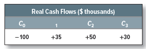
Suppose your firm usually forecasts cash flows in nominal terms and discounts at a 15% nominal rate. In this particular case, however, you are given project cash flows in real terms, that is, current dollars:
It would be inconsistent to discount these real cash flows at the 15% nominal rate. You have two alternatives: Either restate the cash flows in nominal terms and discount at 15%, or restate the discount rate in real terms and use it to discount the real cash flows.
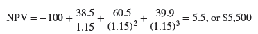
Assume that inflation is projected at 10% a year. Then the cash flow for year 1, which is $35,000 in current dollars, will be 35,000 X 1.10 = $38,500 in year-1 dollars. Similarly, the cash flow for year 2 will be 50,000 X (1.10)2 = $60,500 in year-2 dollars, and so on. If we discount these nominal cash flows at the 15% nominal discount rate, we have
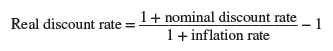
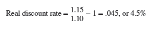
Instead of converting the cash-flow forecasts into nominal terms, we could convert the discount rate into real terms by using the following relationship:
If we now discount the real cash flows by the real discount rate, we have an NPV of $5,500, just as before:
The message of all this is quite simple. Discount nominal cash flows at a nominal discount rate. Discount real cash flows at a real rate. Never mix real cash flows with nominal discount rates or nominal flows with real rates.
4. Rule 4: Separate Investment and Financing Decisions
Suppose you finance a project partly with debt. How should you treat the proceeds from the debt issue and the interest and principal payments on the debt? Answer: You should neither subtract the debt proceeds from the required investment nor recognize the interest and principal payments on the debt as cash outflows. Regardless of the actual financing, you should view the project as if it were all-equity-financed, treating all cash outflows required for the project as coming from stockholders and all cash inflows as going to them.
This procedure focuses exclusively on the project cash flows, not the cash flows associated with alternative financing schemes. It, therefore, allows you to separate the analysis of the investment decision from that of the financing decision. We explain how to recognize the effect of financing choices on project values in Chapter 19.
5. Rule 5: Remember to Deduct Taxes
Taxes are an expense just like wages and raw materials. Therefore, cash flows should be estimated on an after-tax basis. Subtract cash outflows for taxes from pretax cash flows and discount the net amount.
Some firms do not deduct tax payments. They try to offset this mistake by discounting the pretax cash flows at a rate that is higher than the cost of capital. Unfortunately, there is no reliable formula for making such adjustments to the discount rate.
Be careful to subtract cash taxes. Cash taxes paid are usually different from the taxes reported on the income statement provided to shareholders. For example, the shareholder accounts typically assume straight-line depreciation instead of the accelerated depreciation allowed by the U.S. tax code. We will highlight the differences between straight-line and accelerated depreciation later in this chapter.
The next section takes a broader look at corporate income taxes and the recent changes in the U.S. tax code.
he blog was how do i say it… relevant, finally something that helped me. Thanks