The Term Structure of Interest Rates

When we explained in Chapter 2 how to calculate present values, we used the same discount rate to calculate the value of each period’s cash flow. This discount rate was the bond’s yield to maturity y. For many purposes, using a single discount rate is a perfectly acceptable approximation, but there are also occasions when you need to recognize that short-term interest rates may be different from long-term rates. In this case, it may be worth discounting each cash flow at a different rate.

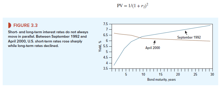
The relationship between short- and long-term interest rates is called the term structure of interest rates. Look, for example, at Figure 3.3, which shows the term structure in two different years. Notice that in the later year, the term structure sloped downward; long-term interest rates were lower than short-term rates. In the earlier year, the pattern was reversed and long-term bonds offered a much higher interest rate than short-term bonds. You now need to learn how to measure the term structure and understand why long- and short-term rates often differ.

Consider a simple loan that pays $1 at the end of one year. To find the present value of this loan you need to discount the cash flow by the one-year rate of interest, r₁:

This rate, r_u is called the one-year spot rate. To find the present value of a loan that pays $1 at the end of two years, you need to discount by the two-year spot rate, r₂:

The first year’s cash flow is discounted at today’s one-year spot rate, and the second year’s flow is discounted at today’s two-year spot rate. The series of spot rates r_b r₂, . . . , r_t, . . . traces out the term structure of interest rates.

Now suppose you have to value $1 paid at the end of years 1 and 2. If the spot rates are different—say, r₁ = 3% and r₂ = 4%—then we need two discount rates to calculate present value:

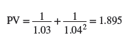
Once we know that PV = 1.895, we can go on to calculate a single discount rate that would give the same answer. That is, we could calculate the yield to maturity by solving for y in the following equation:

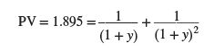
This gives a yield to maturity of 3.66%. Once we have the yield, we could use it to value other two-year annuities. But we can’t get the yield to maturity until we know the price. The price is determined by the spot interest rates for dates 1 and 2. Spot rates come first. Yields to maturity come later, after bond prices are set. That is why professionals often identify spot interest rates and discount each cash flow at the spot rate for the date when the cash flow is received.

1. Spot Rates, Bond Prices, and the Law of One Price

The law of one price states that the same commodity must sell at the same price in a well­functioning market. Therefore, all safe cash payments delivered on the same date must be discounted at the same spot rate.

Table 3.6 illustrates how the law of one price applies to government bonds. It lists three government bonds, which we assume make annual coupon payments. All the bonds have the same coupon but they have different maturities. The shortest (bond A) matures in two years and the longest (bond C) in four.

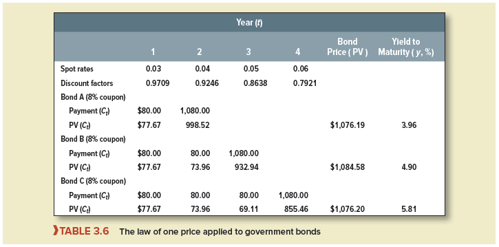
Spot rates and discount factors are given at the top of each column. The law of one price says that investors place the same value on a risk-free dollar regardless of whether it is provided by bond A, B, or C. You can check that the law holds in the table.

Each bond is priced by adding the present values of each of its cash flows. Once total PV is calculated, we have the bond price. Only then can the yield to maturity be calculated.

Notice how the yield to maturity increases as bond maturity increases. The yields increase with maturity because the term structure of spot rates is upward-sloping. Yields to maturity are complex averages of spot rates. For example, you can see that the yield on the four-year bond (5.81%) lies between the one- and four-year spot rates (3% and 6%).

Financial managers who want a quick, summary measure of interest rates bypass spot interest rates and look in the financial press at yields to maturity. They may refer to the yield curve, which plots yields to maturity, instead of referring to the term structure, which plots spot rates. They may use the yield to maturity on one bond to value another bond with roughly the same coupon and maturity. They may speak with a broad brush and say, “Ampersand Bank will charge us 6% on a three-year loan,” referring to a 6% yield to maturity.

Throughout this text, we too use the yield to maturity to summarize the return required by bond investors. But you also need to understand the measure’s limitations when spot rates are not equal.

2. Measuring the Term Structure

You can think of the spot rate, r_t, as the rate of interest on a bond that makes a single payment at time t. Such simple bonds do exist. They are known as stripped bonds, or strips. On request the U.S. Treasury will split a normal coupon bond into a package of mini-bonds, each of which makes just one cash payment. Our 8% bonds of 2021 could be exchanged for eight semiannual coupon strips, each paying $40, and a principal strip paying $1,000. In November 2017, this package of coupon strips would have cost $307.58 and the principal strip would have cost $927.53, making a total cost of $1,235.11, just a little more than it cost to buy one 8% bond. The similarity should be no surprise. Because the two investments provide identical cash payments, they must sell for very close to the same price.

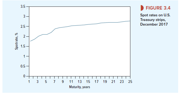
We can use the prices of strips to measure the term structure of interest rates. For example, in November 2017, a 10-year strip cost $793.37. In return, investors could look forward to a single payment of $1,000 in November 2027. Thus, investors were prepared to pay $.79337 for the promise of $1 at the end of 10 years. The 10-year discount factor was DF₁₀ = 1/(1 + r₁₀)¹⁰ = .79337, and the 10-year spot rate was r₁₀ = (1/.79337)¹⁰ – 1 = .0234, or 2.34%. In Figure 3.4, we use the prices of strips with different maturities to plot the term structure of spot rates from 1 to 25 years. You can see that in 2017 investors required a higher interest rate for lending for 25 years rather than for 1.

3. Why the Discount Factor Declines as Futurity Increases—and a Digression on Money Machines

In Chapter 2, we saw that the longer you have to wait for your money, the less is its present value. In other words, the two-year discount factor DF₂ = 1/(1 + r₂)² is less than the one-year discount factor DFj = 1/(1 + r_x). But is this necessarily the case when there can be a different spot interest rate for each period?

Suppose that the one-year spot rate of interest is r₁ = 20% and the two-year spot rate is r₂ = 7%. In this case, the one-year discount factor is DFj = 1/1.20 = .833 and the two-year discount factor is DF₂ = 1/1.07² = .873. Apparently, a dollar received the day after tomorrow is not necessarily worth less than a dollar received tomorrow.

But there is something wrong with this example. Anyone who could borrow and invest at these interest rates could become a millionaire overnight. Let us see how such a “money machine” would work. Suppose the first person to spot the opportunity is Hermione Kraft.

Ms. Kraft first buys a one-year Treasury strip for .833 X $1,000 = $833. Now she notices that there is a way to earn an immediate surefire profit on this investment. She reasons as follows. Next year the strip will pay off $1,000 that can be reinvested for a further year. Although she does not know what interest rates will be at that time, she does know that she can always put the money in a checking account and be certain of having $1,000 at the end of year 2. Her next step, therefore, is to go to her bank and borrow the present value of this $1,000. At 7% interest the present value is PV = 1000/(1.07)² = $873.

So Ms. Kraft borrows $873, invests $830, and walks away with a profit of $43. If that does not sound like very much, notice that by borrowing more and investing more she can make much larger profits. For example, if she borrows $21,778,584 and invests $20,778,584, she would become a millionaire.^[1]

Of course this story is completely fanciful. Such an opportunity would not last long in well-functioning capital markets. Any bank that allowed you to borrow for two years at 7% when the one-year interest rate was 20% would soon be wiped out by a rush of small investors hoping to become millionaires and a rush of millionaires hoping to become billionaires. There are, however, two lessons to our story. The first is that a dollar tomorrow cannot be worth less than a dollar the day after tomorrow. In other words, the value of a dollar received at the end of one year (DF₁) cannot be less than the value of a dollar received at the end of two years (DF₂). There must be some extra gain from lending for two periods rather than one: (1 + r₂)² cannot be less than 1 + r_x.

Our second lesson is a more general one and can be summed up by this precept: “There is no such thing as a surefire money machine.” The technical term for money machine is arbitrage. In well-functioning markets, where the costs of buying and selling are low, arbitrage opportunities are eliminated almost instantaneously by investors who try to take advantage of them.

Later in the book we invoke the absence of arbitrage opportunities to prove several useful properties about security prices. That is, we make statements like, “The prices of securities X and Y must be in the following relationship—otherwise there would be potential arbitrage profits and capital markets would not be in equilibrium.”

Source:  Brealey Richard A., Myers Stewart C., Allen Franklin (2020), Principles of Corporate Finance, McGraw-Hill Education; 13th edition.