1. Some Tricks of the Trade
Sangria had just one asset and two sources of financing. A real company’s market-value balance sheet has many more entries, for example:
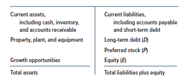
Several questions immediately arise:
How does the formula change when there are more than two sources of financing?
Easy: There is one cost for each element. The weight for each element is proportional to its market value. For example, if the capital structure includes both preferred and common shares,
![]()
where rP is investors’ expected rate of return on the preferred stock, P is the amount of preferred stock outstanding, and V = D + P + E.
What about short-term debt? Many companies consider only long-term financing when calculating WACC. They leave out the cost of short-term debt. In principle, this is incorrect. The lenders who hold short-term debt are investors who can claim their share of operating earnings. A company that ignores this claim will misstate the required return on capital investments.
But “zeroing out” short-term debt is not a serious error if the debt is only temporary, seasonal, or incidental financing or if it is offset by holdings of cash and marketable securities. Suppose, for example, that one of your foreign subsidiaries takes out a six-month loan to finance its inventory and accounts receivable. The dollar equivalent of this loan will show up as a short-term debt. At the same time, headquarters may be lending money by investing surplus dollars in short-term securities. If this lending and borrowing offset, there is no point in including the cost of short-term debt in the weighted-average cost of capital, because the company is not a net short-term borrower.
What about other current liabilities? Current liabilities are usually “netted out” by subtracting them from current assets. The difference is entered as net working capital on the left-hand side of the balance sheet. The sum of long-term financing on the right is called total capitalization.
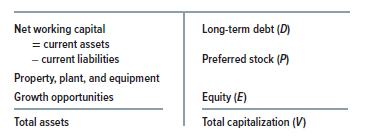
When net working capital is treated as an asset, forecasts of cash flows for capital investment projects must treat increases in net working capital as a cash outflow and decreases as an inflow. This is standard practice, which we followed in Section 6-2. We also did so when we estimated the future investments that Rio would need to make in working capital.
Because current liabilities include short-term debt, netting them out against current assets excludes the cost of short-term debt from the weighted-average cost of capital. We have just explained why this can be an acceptable approximation. But when short-term debt is an important, permanent source of financing—as is common for small firms and firms outside the United States—it should be shown explicitly on the right-hand side of the balance sheet, not netted out against current assets.[1] The interest cost of short-term debt is then one element of the weighted-average cost of capital.
How are the costs of financing calculated? You can often use stock market data to get an estimate of rE, the expected rate of return demanded by investors in the company’s stock. With that estimate, WACC is not too hard to calculate because the borrowing rate rD and the debt and equity ratios D/V and E/V can be directly observed or estimated without too much trouble.[2] Estimating the value and required return for preferred shares is likewise usually not too complicated.
Estimating the required return on other security types can be troublesome. Convertible debt, where the investors’ return comes partly from an option to exchange the debt for the company’s stock, is one example. We leave convertibles to Chapter 24.
Junk debt, where the risk of default is high, is likewise difficult. The higher the odds of default, the lower the market price of the debt, and the higher is the promised rate of interest. But the weighted-average cost of capital is an expected—that is, average—rate of return, not a promised one. For example, as we write this in 2018, the three-year bonds issued by Bon-Ton Department Stores are priced at 12.5%% of face value and offer a promised yield of 110%, about 108 percentage points above yields on the highest-quality debt issues maturing at the same time. The price and yield on the Bon-Ton bond demonstrated investors’ concern about the company’s chronic financial ill-health. But the 110% yield was not an expected return because it did not average in the losses to be incurred if the company were to default. Including 110% as a “cost of debt” in a calculation of WACC would therefore have overstated Bon-Ton’s true cost of capital.
This is bad news: There is no easy way of estimating the expected rate of return on most junk debt issues. The good news is that for most debt, the odds of default are small. That means the promised and expected rates of return are close, and the promised rate can be used as an approximation in calculating the weighted-average cost of capital.
Should I use a company or industry WACC? Of course, you want to know what your company’s WACC is. Yet industry WACCs are sometimes more useful. Here’s an example. Kansas City Southern used to be a portfolio of (1) the Kansas City Southern Railroad, with operations running from the U.S. Midwest south to Texas and Mexico, and (2) Stillwell Financial, an investment-management business that included the Janus mutual funds. It’s hard to think of two more dissimilar businesses. Kansas City Southern’s overall WACC was not right for either of them. The company would have been well advised to use a railroad industry WACC for its railroad operations and an investment management WACC for Stillwell.[3]
Kansas City Southern spun off Stillwell in 2000 and is now a pure-play railroad. But even now, the company would be wise to check its WACC against a railroad industry WACC. Industry WACCs are less exposed to random noise and estimation errors. Fortunately for Kansas City Southern, there are five large, pure-play railroads (including Canadian Pacific and Canadian National Railway) that the company could use to calculate an industry WACC. Of course, use of an industry WACC for a particular company’s investments assumes that the company and industry have approximately the same business risk. Industry WACCs also have to be adjusted (by the three-step procedure given below) if industry-average debt ratios differ from the target debt ratio for the project to be valued.
Don’t use industry WACCs blindly. Railroad companies are relatively homogenous, and therefore it may be helpful to look at a railroad WACC. But an industry-average WACC for Miscellaneous Consumer Goods would be almost useless as a guide to the WACC of an individual company.[4]
What tax rate should I use? Taxes are complicated. Corporations can often reduce average tax rates by taking advantage of special provisions (some might say “loopholes”) in the
tax code. But the WACC formula calls for the marginal tax rate—that is, the cash taxes paid as a percentage of each dollar of additional income generated by a capital-investment project.
The examples in this chapter use 21%, the current U.S. space corporate rate. In practice, U. S. corporations add three or four percentage points to cover state taxation. Thus, a corporation operating nationwide—and paying income taxes in most states—might use a 24% or 25% rate to calculate WACC.
What if the company can’t use all its interest tax shields? So far, we have assumed that the company is consistently profitable and will pay taxes at the full statutory rate, which in the United States is now 21%. Thus, the company can still use a new project’s depreciation tax shields even if a project endures a period of start-up losses. The project’s depreciation expense shields some of the company’s overall taxable income. Interest tax shields on debt supported by the new project can be captured in the same way.
Sometimes interest tax shields from new debt cannot be captured immediately because (1) the company is suffering losses overall or (2) its total interest payments exceed 30% of EBITDA.[5] Should the company change its WACC if it finds itself in one or both of these unfortunate states?
Probably not, if the losses or constraint are temporary. Tax losses and nondeductible interest can be carried forward and used to shield future income. (The tax rate in the WACC formula could be reduced to account for delay in using tax shields.) But if the wait to use interest tax shields from additional borrowing is long enough, it may be best to use the APV method, which we explain in the next section.
2. Adjusting WACC When Debt Ratios and Business Risks Differ
The WACC formula assumes that the project or business to be valued will be financed in the same debt-equity proportions as the company (or industry) as a whole. What if that is not true? For example, what if Sangria’s perpetual crusher project supports only 20% debt, versus 40% for Sangria overall?
Moving from 40% to 20% debt may change all the inputs to the WACC formula.[6] Obviously, the financing weights change. But the cost of equity rE is less because financial risk is reduced. The cost of debt may be lower, too.
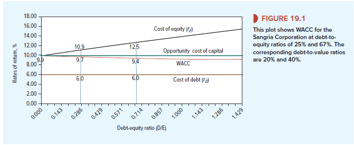
Take a look at Figure 19.1, which plots Sangria’s WACC and the costs of debt and equity as a function of its debt-equity ratio. The flat line is r, the opportunity cost of capital. Remember, this is the expected rate of return that investors would want from the company if it were all-equity-financed. The opportunity cost of capital depends only on business risk and is the natural reference point.
Suppose Sangria or the perpetual crusher project were all-equity-financed (D/V = 0). At that point, WACC and the opportunity cost of capital are identical. Start from that point in Figure 19.1. As the debt ratio increases, the cost of equity increases because of financial risk, but notice that WACC declines. The decline is not caused by use of “cheap” debt in place of “expensive” equity. It falls because of the tax shields on debt interest payments. If there were no corporate income taxes, the weighted-average cost of capital would be constant and equal to the opportunity cost of capital at all debt ratios. We showed this in Chapter 17.
Figure 19.1 shows the shape of the relationship between financing and WACC, but initially we have numbers only for Sangria’s current 40% debt ratio. We want to recalculate WACC at a 20% ratio.
Here is the simplest way to do it. There are three steps.
Step 1 Calculate the opportunity cost of capital. In other words, calculate WACC and the cost of equity at zero debt. This step is called unlevering the WACC. The simplest unlevering formula is
![]()
This formula comes directly from Modigliani and Miller’s proposition 1 (see Section 17-1). If taxes are left out, the weighted-average cost of capital equals the opportunity cost of capital and is independent of leverage.
Step 2 Estimate the cost of debt, rD, at the new debt ratio, and calculate the new cost of equity.
![]()
This formula is Modigliani and Miller’s proposition 2 (see Section 17-2). It calls for D/E, the ratio of debt to equity, not debt to value.
Step 3 Recalculate the weighted-average cost of capital at the new financing weights.
Let’s do the numbers for Sangria at D/V = .20, or 20%.
Step 1. Sangria’s current debt ratio is D/V = .4. So the opportunity cost of capital is:
r = .06(.4) + .125(.6) = .099, or 9.9%
Step 2. We will assume that the debt cost stays at 6% when the debt ratio is 20%. Then
rE = .099 + (.099 – .06)(.25) = .109, or 10.9%
Note that the debt-equity ratio is .2/.8 = .25.
Step 3. Recalculate WACC.
WACC = .06(1 – .21)(.2) + .109(.8) = .097, or 9.7%
Figure 19.1 enters these numbers on the plot of WACC versus the debt-equity ratio.
3. Unlevering and Relevering Betas
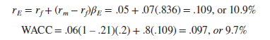
Our three-step procedure (1) unlevers and then (2) relevers the cost of equity. Some financial managers find it convenient to (1) unlever and then (2) relever the equity beta. Given the beta of equity at the new debt ratio, the cost of equity can be calculated from the capital asset pricing model. We can then compute the WACC at the new debt ratio.
Suppose Sangria’s debt and equity betas in our example are pD = .135 and pE = 1.07.14 If the risk-free rate is 5%, and the market risk premium is 7.0%, then Sangria’s cost of equity is
![]()
This matches the cost of equity in our example at a 40/60 debt-equity ratio.
To find Sangria’s weighted average cost of capital at a 20% debt ratio, we can follow a three-step procedure that pretty much matches the procedure that we used earlier.
Step 1 Unlever beta. The unlevered beta is the beta of the equity if the company had zero debt. The formula for unlevering beta was given in Section 17-2.
![]()
This equation says that the beta of a firm’s assets (pA) is equal to the beta of a portfolio of all of the firm’s outstanding debt and equity securities. An investor who bought such a portfolio would own the assets free and clear and absorb only business risks. For Sangria,
![]()
Step 2 Estimate the betas of the debt and equity at the new debt ratio. The formula for relevering beta closely resembles MM’s proposition 2, except that betas are substituted for rates of return:
![]()
Use this formula to recalculate pE when D/E changes. If the beta of Sangria’s debt stays at .135 when it moves to a debt-equity ratio of .2/.8 =.25, then
![]()
Step 3 Recalculate the cost of equity and the WACC at the new financing weights:
This corresponds to the figure that we calculated above and plotted in Figure 19.1.
4. The Importance of Rebalancing
The formulas for WACC and for unlevering and relevering expected returns are simple, but we must be careful to remember the underlying assumptions. The most important point is rebalancing.
Calculating WACC for a company at its existing capital structure requires that the capital structure won’t change; in other words, the company must rebalance its capital structure to maintain the same market-value debt ratio for the relevant future. Take Sangria Corporation as an example. It starts with a debt-to-value ratio of 40% and a market value of $1,250 million. Suppose that Sangria’s products do unexpectedly well in the marketplace and that market value increases to $1,500 million. Rebalancing means that it will then increase debt to .4 x 1,500 = $600 million, thus regaining a 40% ratio. The proceeds of the additional borrowing could be used to finance other investments or it could be paid out to the stockholders. If market value instead falls, Sangria would have to pay down debt proportionally.
Of course, real companies do not rebalance capital structure in such a mechanical and compulsive way. For practical purposes, it’s sufficient to assume gradual but steady adjustment toward a long-run target.[7] But if the firm plans significant changes in capital structure (for example, if it plans to pay off its debt), the WACC formula won’t work. In such cases, you should turn to the APV method, which we describe in the next section.
Our three-step procedure for recalculating WACC with a different debt ratio makes a similar rebalancing assumption.[8] Whatever the starting debt ratio, the firm is assumed to rebalance to maintain that ratio in the future.[9]
5. The Modigliani-Miller Formula, Plus Some Final Advice
What if the firm does not rebalance to keep its debt ratio constant? In this case, the only general approach is adjusted present value, which we cover in the next section. But sometimes financial managers turn to other discount-rate formulas, including one derived by Modigliani and Miller (MM). MM considered a company or project generating a level, perpetual stream of cash flows financed with fixed, perpetual debt. There is then a simple relationship between the after-tax discount rate (rMM) and the opportunity cost of capital (r):[10]
![]()
Here it’s easy to unlever: just set the debt-capacity parameter (D/V) equal to zero.19
MM’s formula is still used in practice, but it is exact only in the special case where there is a level, perpetual stream of cash flows and fixed, perpetual debt. However, the formula is not a bad approximation for projects that are not perpetual as long as debt is issued in a fixed amount.20
So which team do you want to play with, the fixed-debt team or the rebalancers? If you join the fixed-debt team you will be outnumbered. Most financial managers use the plain, after-tax WACC, which assumes constant market-value debt ratios and therefore assumes rebalancing. That makes sense, because the debt capacity of a firm or project must depend on its future value, which will fluctuate.
At the same time, we must admit that the typical financial manager doesn’t care much if his or her firm’s debt ratio drifts up or down within a reasonable range of moderate financial leverage. The typical financial manager acts as if a plot of WACC against the debt ratio is “flat” (constant) over this range. This too makes sense, if we just remember that interest tax shields are the only reason why the after-tax WACC declines in Figures 17.4 and 19.1. The WACC formula doesn’t explicitly capture costs of financial distress or any of the other non-tax complications discussed in Chapter 18.21 All these complications may roughly cancel the value added by interest tax shields (within a range of moderate leverage). If so, the financial manager is wise to focus on the firm’s operating and investment decisions, rather than on fine-tuning its debt ratio.
Hello my family member! I wish to say that this article is awesome, nice written and come with approximately all important infos. I¦d like to peer more posts like this .