To calculate the weighted-average cost of capital, you need an estimate of the cost of equity. You decide to use the capital asset pricing model (CAPM). Here you are in good company: As we saw in the last chapter, most large U.S. companies do use the CAPM to estimate the cost of equity, which is the expected rate of return on the firm’s common stock.[1] The CAPM says that
![]()
Now you have to estimate beta. Let us see how that is done in practice.
1. Estimating Beta
In principle, we are interested in the future beta of the company’s stock, but lacking a crystal ball, we turn first to historical evidence. For example, look at the scatter diagram at the top left of Figure 9.2. Each dot represents the return on U.S. Steel stock and the return on the market in a particular month. The plot starts in January 2008 and runs to December 2012, so there are 60 dots in all.
The second diagram on the left shows a similar plot for the returns on Microsoft stock, and the third shows a plot for Consolidated Edison. In each case, we have fitted a line through the points. The slope of this line is an estimate of beta. It tells us how much on average the stock price changed when the market return was 1% higher or lower.
The right-hand diagrams show similar plots for the same three stocks during the subsequent period ending in December 2017. The estimated betas are not constant. For example, the estimate for U.S. Steel is much lower in the first period than in the second. You would have been off target if you had blindly used its beta during the earlier period to predict its beta in the later years. However, you could have been pretty confident that ConEd’s beta was much less than U.S. Steel’s and that Microsoft’s beta was somewhere between the two.5
Only a portion of each stock’s total risk comes from movements in the market. The rest is firm-specific, diversifiable risk, which shows up in the scatter of points around the fitted lines in Figure 9.2. R-squared (R2) measures the proportion of the total variance in the stock’s returns that can be explained by market movements. For example, from 2013 to 2017, the R2 for Microsoft was .20. In other words, 20% of Microsoft’s risk was market risk and 80% was diversifiable risk.6 The variance of the returns on Microsoft stock was 439.7 So we could say that the variance in stock returns that was due to the market was .2 x 439 = 88, and the variance of diversifiable returns was .80 x 439 = 351.
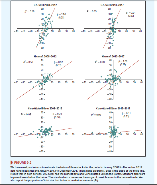
The estimates of beta shown in Figure 9.2 are just that. They are based on the stocks’ returns in 60 particular months. The noise in the returns can obscure the true beta.8 Therefore, statisticians calculate the standard error of the estimated beta to show the extent of possible mismeasurement. Then they set up a confidence interval of the estimated value plus or minus two standard errors. We can be much more confident of some estimates than of others. For example, the standard error on Microsoft’s estimated beta in the second period is 0.26. Thus, the confidence interval for the beta is 1.00 plus or minus 2 x .26. If you state that the true beta for Microsoft is between .48 and 1.52, you have a 95% chance of being right. We can be much less confident of our estimate of U.S. Steel’s beta in the 2013-2017 period. Its standard error is .93. So the true beta for U.S. Steel could well be much lower than our estimated figure of 3.01.9
Usually, you will have more information (and thus more confidence) than this simple, and somewhat depressing, calculation suggests. For example, you know that ConEd’s estimated beta was well below 1 in two successive five-year periods. U.S. Steel’s estimated beta was well above 1 in both periods. Nevertheless, there is always a large margin for error when estimating the beta for individual stocks.
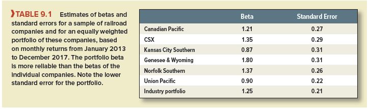
Fortunately, the estimation errors tend to cancel out when you estimate betas of portfolios.10 That is why financial managers often turn to industry betas. For example, Table 9.1 shows estimates of beta and the standard errors of these estimates for the common stocks of six railroad companies. The standard errors are for the most part close to .3. However, the table also shows the estimated beta for a portfolio of all six railroad stocks. Notice that the estimated industry beta is somewhat more reliable. This shows up in the lower standard error.
2. The Expected Return on CSX’s Common Stock
Suppose that in January 2018 you had been asked to estimate the company cost of capital of CSX. Table 9.1 provides two clues about the true beta of CSX’s stock: the direct estimate of 1.35 and the average estimate for the industry of 1.25. We will use the industry estimate of 1.25.
The next issue is what value to use for the risk-free interest rate. In early 2018, the three- month Treasury bill rate was about 1.6%. The one-year interest rate was a little higher, at 2.0%. Yields on longer-maturity U.S. Treasury bonds were higher still, at about 3.0% on 20-year bonds.
The CAPM is a short-term model. It works period by period and calls for a short-term interest rate. But could a 1.6% three-month risk-free rate give the right discount rate for cash flows 10 or 20 years in the future? Well, now that you mention it, probably not.
Financial managers muddle through this problem in one of two ways. The first way simply uses a long-term risk-free rate in the CAPM formula. If this short-cut is used, then the market risk premium must be restated as the average difference between market returns and returns on long-term Treasuries.
The second way retains the usual definition of the market risk premium as the difference between market returns and returns on short-term Treasury bill rates. But now you have to forecast the expected return from holding Treasury bills over the life of the project. In Chapter 3, we observed that investors require a risk premium for holding long-term bonds rather than bills. Table 7.1 showed that over the past century, this risk premium has averaged about 1.5%. So to get a rough but reasonable estimate of the expected long-term return from investing in Treasury bills, we need to subtract 1.5% from the current yield on long-term bonds. In our example
Expected long-term return from bills = yield on long-term bonds – 1.5%
= 3.0 – 1.5 = 1.5%
This is a plausible estimate of the expected average future return on Treasury bills. We therefore use this rate in our example.
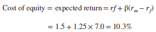
Returning to our CSX example, suppose you decide to use a market risk premium of 7%. Then the resulting estimate for CSX’s cost of equity is about 10.3%:
3. CSX’s After-Tax Weighted-Average Cost of Capital
Now you can calculate CSX’s after-tax WACC. The company’s cost of debt was about 4.0%. With a 21% corporate tax rate, the after-tax cost of debt was rD(1 – TC) = 4.0 X (1 – .21) = 3.2%. The ratio of debt to overall company value was D/V = 19.2%. Therefore
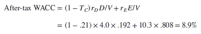
CSX should set its overall cost of capital to 8.9%, assuming that its CFO agrees with our estimates.
Warning The cost of debt is always less than the cost of equity. The WACC formula blends the two costs. The formula is dangerous, however, because it suggests that the average cost of capital could be reduced by substituting cheap debt for expensive equity. It doesn’t work that way! As the debt ratio D/V increases, the cost of the remaining equity also increases, offsetting the apparent advantage of more cheap debt. We show how and why this offset happens in Chapter 17.
Debt does have a tax advantage, however, because interest is a tax-deductible expense. That is why we use the after-tax cost of debt in the after-tax WACC. We cover debt and taxes in much more detail in Chapters 18 and 19.
4. CSX’s Asset Beta
The after-tax WACC depends on the average risk of the company’s assets, but it also depends on taxes and financing. It’s easier to think about project risk if you measure it directly. The direct measure is called the asset beta.
We calculate the asset beta as a blend of the separate betas of debt (pD) and equity (pE). For CSX, we have pE = 1.25, and we’ll assume pD = .15.[4] The weights are the fractions of debt and equity financing, D/V = .192 and E/V = .808:
Calculating an asset beta is similar to calculating a weighted-average cost of capital. The debt and equity weights D/V and E/V are the same. The logic is also the same: Suppose you purchased a portfolio consisting of 100% of the firm’s debt and 100% of its equity. Then you would own 100% of its assets lock, stock, and barrel, and the beta of your portfolio would equal the beta of the assets. The portfolio beta is of course just a weighted average of the betas of debt and equity.
This asset beta is an estimate of the average risk of CSX’s railroad business. It is a useful benchmark, but it can take you only so far. Not all railroad investments are average risk. And if you are the first to use railroad-track networks as interplanetary transmission antennas, you will have no asset beta to start with.
How can you make informed judgments about costs of capital for projects or lines of business when you suspect that risk is not average? That is our next topic.
Hi there, I found your site by the use of Google whilst searching for a comparable subject, your website came up, it looks good. I’ve bookmarked it in my google bookmarks.