1. EXAMINING RESIDUALS
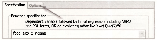
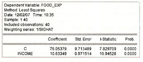
In this chapter we return to the example considered in Chapters 2 to 4 where weekly expenditure on food was related to income. Data in the file food.wfl were used to find the following least squares estimates.
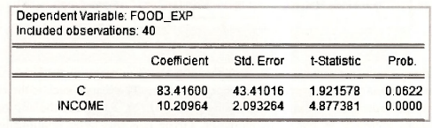
We are now concerned with whether the error variance for this equation is likely to vary over observations, a characteristic called heteroskedasticity. To carry out a preliminary investigation of this question, we examine the least squares residuals. If they increase with increasing income, that suggests the error variance increases with income.
1.1. Plot against observation number
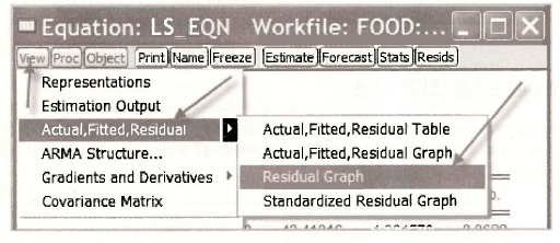
There are a variety of ways in which EViews can be used to examine least squares residuals. Let us begin by checking the obvious ones. After estimating the equation and naming it ls_eqn, go to View/Actual, Fitted, Residual. At that point you will see a menu with the following options.
Actual, Fitted, Residual Table
Actual, Fitted, Residual Graph
Residual Graph
Standardized Residual Graph
Check each of these options to get a feel for the different ways in which they convey information. As you might expect from the names of the options, each alternative presents information on one or more of the series actual, fitted and residual. In terms of the names of the series in your workfile
The Standardized Residual Graph is a graph of e/a; the residuals have been standardized (made free of units of measurement) by dividing by the estimated standard deviation of the error term.
In each case the series are graphed against the observation number. As an example, consider the Residual Graph selected in the following way.
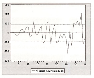
In the residual graph that follows it is clear that the absolute magnitude of the residuals has a tendency to be larger as the observation number gets larger. The reason such is the case is that the observations are ordered according to increasing values of INCOME, and the absolute magnitude of the residuals increases as INCOME increases. Given it is this latter relationship that we are really interested in, it is preferable to graph the residuals against income. Nevertheless, residual graphs like the one below are important for examining which observations are not well captured by the estimated model (outliers), and, in the case of time series data, for discerning patterns in the residuals. To help you assess which observations could be viewed as outliers, dotted lines are drawn at points one standard deviation (a = 89.517 ) either side of zero.
1.2. Plot against an explanatory variable
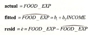
To graph the residuals against income we begin by naming the residuals and the fitted values.
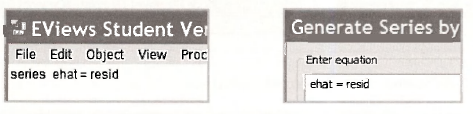
series ehat = resid
series foodhat = food exp – ehat
Recall that these commands can be executed by typing them in the upper EViews window or by clicking on Genr and writing the equation to generate the series in the resulting box. Examples of these two alternatives for the first command follow.
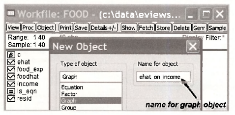
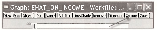
Returning to our task of graphing the residuals, we create a graph object by going to Object/ New Object and selecting Graph. As a name for the graph, we chose EHAT_ON_INCOME.
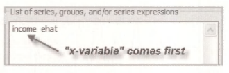
After clicking OK, you will be asked for the series that you want to graph. The one that is to go on the x-axis comes first.
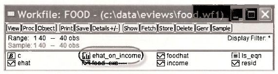
After clicking OK one more time, a graph object will appear in your workfile.
Double clicking on this object will open it. Be careful, however. It may not look like you expected! Unless told otherwise, EViews will assume you want both INCOME and EHAT graphed against the observation number. You need to tell EViews to change the graph so that INCOME is on the x-axis and EHA T is on the y-axis. Also, given that income is not measured in equally spaced intervals, dots are preferred to a line graph. With these factors in mind, open the graph and select Options.
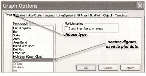
Then select Type/Scatter, click Apply, and click OK.
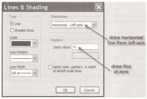
A nice looking scatter plot will appear. You can make it look even nicer by drawing a horizontal line at zero. Select Line/Shade.

Fill in the resulting dialog box as follows.
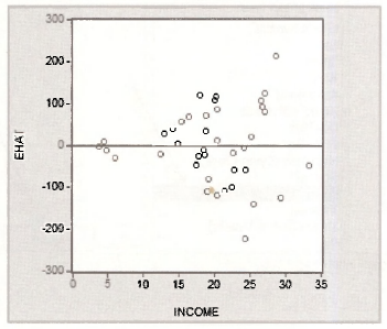
Clicking OK gives the required graph. Notice how the absolute magnitude of the residuals is larger for larger values of income, an indication of heteroskedasticity.
1.3. Plot of least squares line
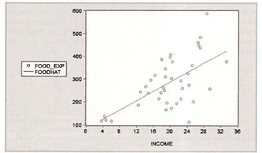
Another way to illustrate the dependence of the magnitude of the residuals on INCOME is to plot FOOD EXP and the least-squares estimated line against INCOME, as is displayed in Figure 8.2 on page 200 of the text. To reproduce this figure, select Object/New Object/Graph and give the graph a name, say FIGURE 8 2.
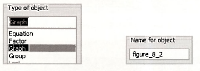
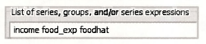
The relevant three variables for the graph are INCOME, FOOD EXP and FOODHAT, with FOODHAT being required to draw the least-squares estimated line. The x-axis variable INCOME is listed first.
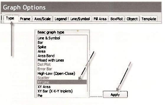
After clicking OK, a graph will appear in your workfile. Several adjustments are needed to this graph to convert it to the one we want. The process is slightly complicated because we want a line graph for FOODHAT, but we want dots or symbols for FOOD EXP. The strategy that we adopt is to ask for line graphs first, and then change the one for FOOD EXP to dots. With these points in mind, open the graph object FIGURE_8_2 and select Options/Type/XY Line. Click Apply.
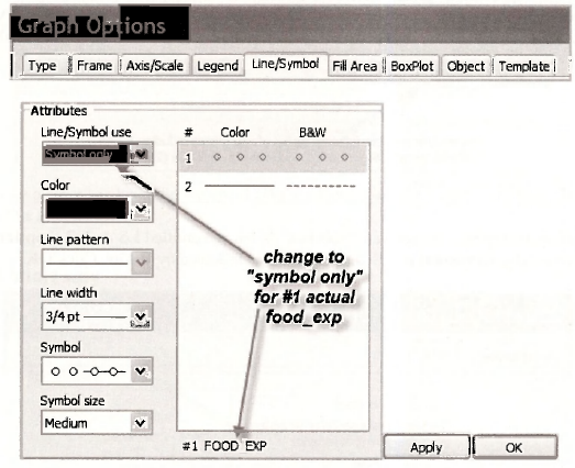
Then select Line/Symbol. The snapshot below shows you how you change the line for FOOD EXP to dots (symbols). No changes are needed for series #2, FOODHAT. It is already represented by the required line. Click Apply. Click OK.
The graph object FIGURE_8_2 will now appear as follows. Compare it with Figure 8.2 in the text. Other changes can be made. We could label the line, and we could change the legend, that at present appears in a box on the left of the graph. We suggest you experiment with these options. For labeling, select the button [AddText], For changing the legend, go to Options/ Legend. You can also cut and paste it into a document using Ctrl+C followed by Ctrl+V.
2. HETEROSKEDASTICITY-CONSISTENT STANDARD ERRORS
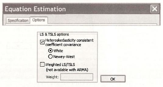
One option for correcting conventional least-squares interval estimates and hypothesis tests that are no longer appropriate under heteroskedasticity is to use what are known as White’s heteroskedasticity-consistent standard errors. These standard errors are obtained in EViews by choosing an estimation option. In the Equation Estimation box, click on the Options tab.
In the Options dialog box, the relevant “sub-box” is the one entitled LS & TSLS options. Select Heteroskedasticity consistent coefficient covariance followed by White. Click OK.
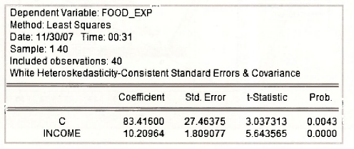
In the output that follows there is a note telling you that the standard errors and covariance are the heteroskedasticity-consistent ones. By “covariance”, it means the whole covariance matrix for the estimated coefficients. The standard errors are the square roots of the diagonal elements of this matrix. All test outcomes computed from this new object, including the Wald tests considered extensively in Chapter 6, will use the new covariance matrix. The least squares estimates remain the same. See page 202 of the text.
3. WEIGHTED LEAST SQUARES
In Section 8.3.1 of the text the regression error variance is assumed to be heteroskedastic of the form σ2 = σ2xj where xj = INCOMEi. Under this specification the minimum variance unbiased estimator for the regression coefficients (β1, and β2 is the generalized least squares estimator. This estimator is also known as the weighted least squares estimator where, in this case, each observation is weighted by
There are two ways to obtain the weighted least squares estimator, a short way and a long way. It is instructive to consider both.
3.1. A short way
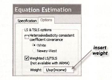
Weighted least squares is another Equation Estimation option, so our starting point is the same as that for the White standard errors, namely
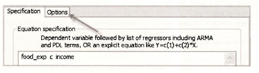
In this case, however, we select Weighted LS/TSLS from the LS & TSLS options. In the Weight box we type 1/sqr(income), where sqr is the EViews function for square root
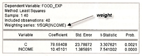
Check the output that follows. You will discover that it coincides with that given on page 204 of the text. You can tell that weighted least squares is the estimation procedure from the line that says Weighting series: 1/SQR(INCOME).
3.2. A long way
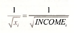
The long way to obtain weighted least squares estimates is to transform each of your variables by dividing by √INCOME as described on page 203 of the text, and to then apply least squares without the weights. The variables can be transformed by creating new series, or by dividing each variable by √INCOME in the equation specification. If you choose to create new series, the following commands are suitable.
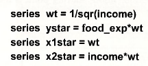
Enter these new series in the Equation specification box
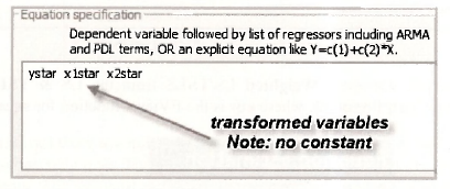
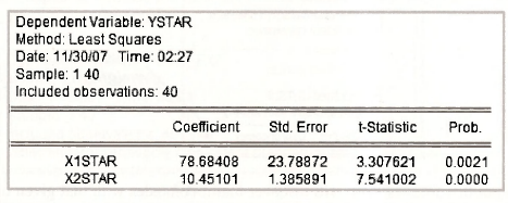
Click OK. Observe that the resulting estimates are the same as those we obtained the short way.
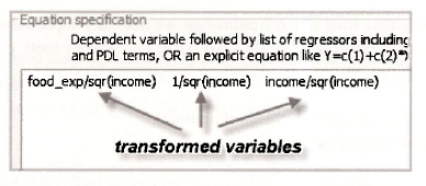
An alternative way that avoids the need to define new series is to transform the variables within the Equation specification, as illustrated below. Try it. Check your output.
4. ESTIMATING A VARIANCE FUNCTION
The heteroskedastic assumption made in the previous section (σ2i =σ2x ) can be viewed as a special case of the more general assumption σ²i = σ2xyi] where y is an unknown parameter. Under this more general assumption y must be estimated before we can proceed with weighted or generalized least squares estimation. In line with Section 8.3.2 of the text (page 205), we first estimate σ2 and y and then proceed to generalized least squares estimation.
4.1. Variance function estimates
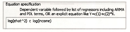
The equation for estimating σ2 and y is written as
![]()
where ei are the least squares residuals, a, = ln(σ2) and a2 -y . Recognizing that the ei, were previously saved in the workfile food.wfl under the name EH AT, and that xi – INCOME, least squares estimates for a1 and a2 are obtained using the following Equation specification.
The resulting output coincides with the results on page 206 of the text.
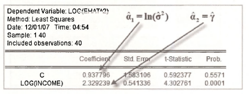
To proceed to generalized least squares estimation we need the exponential of the predictions from this equation, σ2i =exp(a1 + a2 In(INCOMEi)) or their square roots σi . It is instructive to consider two ways of computing them. The first is using the commands

As long as the variance equation is the most recent regression model that has been estimated, in the first of these commands C(1) = a1, and C(2) = a2
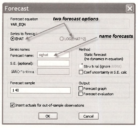
An alternative way of obtaining ct; = sighat is to use the forecast option. In the window displaying the output from estimating the variance equation, click on [Forecast], in the resulting forecast window, you will see two possible series that can be forecast, EHAT and LOG(EHATˆ2). This choice has arisen because the dependent variable in the Equation specification was written as log(e2), a transformation of the series e . EViews is giving you the option of forecasting the original series e or its transformed version log(e2). If you had defined the dependent variable as q = log(e2) via a series command, and then specified your dependent variable as q, EViews would not have been given you a choice. It would assume you want to forecast q. Writing the transformation as part of the equation specification is what leads to the choice.
Now consider the two options. If you click LOG(EHATˆ2), EViews will give you the forecasts qi = In(σ2i). If you click EHAT, it will invert the transformation given in the Equation specification and give you the forecasts σi = √exp(qi) . Since it is σi, that is needed to transform the variables in the generalized least squares procedure, we choose EHAT. We call the forecast series SIGHAT.
4.2. Generalized least squares
To obtain the generalized least squares estimates in equation (8.27) on page 207 of the text we can use EViews weighted least squares option, with weighting series σ-1 = 1/SIGHAT. The Equation specification and LS & TSLS options are given by
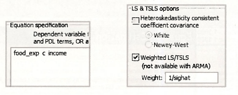
These selections yield the following output.
5. A HETEROSKEDASTIC PARTITION
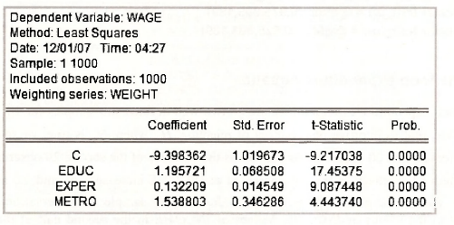
In Section 8.3.3 of the text we use data from the file cps2.dat to estimate the equation
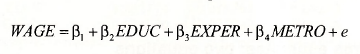
We are hypothesizing that WAGE depends on education (EDUC), experience (EXPER), and whether a worker lives in a metropolitan area ( METRO = 1 for metropolitan area, METRO = 0 for rural area). Three sets of estimates are obtained: (1) a least-squares regression on all observations, (2) two separate least-squares regressions, one for metropolitan workers and one for rural workers, and (3) a generalized least-squares regression that uses all observations, but which assumes the error variances for metropolitan and rural workers are different. This latter assumption is referred to as a “heteroskedastic partition”.
5.1. Least-squares estimates: one equation
No new features of EViews are required for single equation least-squares estimation of the wage equation. However, we report the equation specification and the output for completeness.
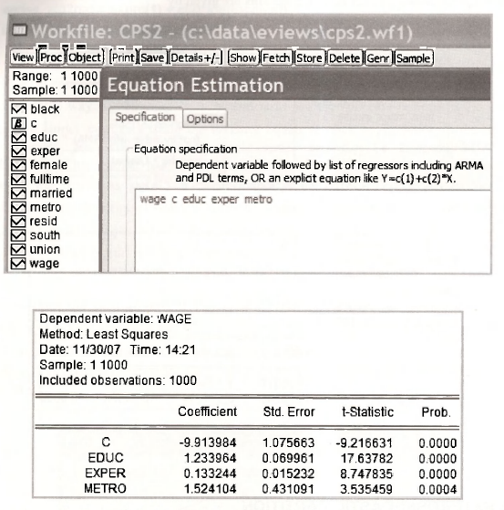
Check these results against those in equation (8.28) on page 208 of the text.
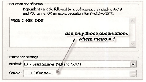
5.2. Least-squares estimates: two equations
To estimate two separate equations, one for metropolitan workers and one for rural workers, we use EViews to restrict the sample to the relevant observations. For the metropolitan observations, we change the sample by going to the Estimation settings box and specifying
sample 1 1000 if metro = 1
This instruction tells EViews to consider all 1000 observations, but to restrict estimation to those where metro = 1.
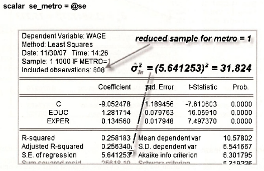
The results follow. Notice that EViews reminds you about the sample you have chosen and it also tells you how many observations satisfy the restriction that you imposed for their inclusion. We have 808 metropolitan observations. The estimates are consistent with those on page 209 of the text. Of particular interest are the standard deviation and variance of the error term, σM =5.641 and σ2M =31.824. They are needed for the generalized least squares estimates in the next section.
The value σM =5.641 is stored temporarily as @se; we can save it as se_metro using the command
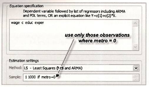
The same steps are followed for the rural observations, but in this case we restrict the sample to those observations where metro = 0.
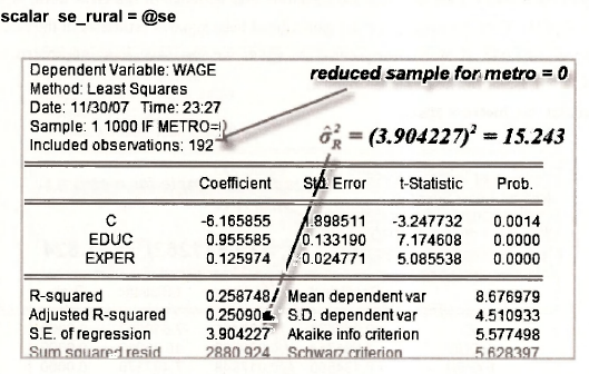
The results below show that there are 192 rural observations. The standard deviation and variance of the error term are, respectively, σR = 3.904 and σ2R = 15.243 . We save the value for aK using the command
5.3. Generalized least-squares estimates
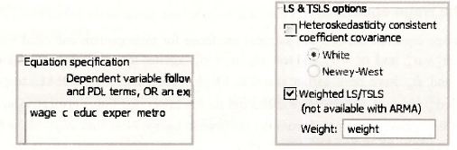
For generalized least squares estimation we can use EViews weighted least squares option with the weighting series equal to cr^ for the metropolitan observations and a“‘ for the rural observations. Thus, we create the series
series weight = metro*(1/se_metro) + (1-metro)*(1/se_rural)
The relevant equation and option specifications are
The following results can be checked against those on page 210 of the text.
6. THE GOLDFELD-QUANDT TEST
As tests for heteroskedasticity we consider a test known as the Goldfeld-Quandt test and a general class of tests based on an estimated variance function. The statistic for the Goldfeld-Quandt test is the ratio of error variance estimates from two sub-samples of the observations. If those estimates are σ21 and σ22 , obtained from sub-sample regressions with (N1 -K1) and (N2 -K2) degrees of freedom, respectively, then, under the null hypothesis H0: σ21 = σ22
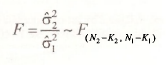
If the alternative hypothesis is H1: σ21 # σ22, and a 5% significance level is used, the test is a two- tail one with critical values F(0975. N2 -K2, N1 -K1 ) and ![]() . For a 5% one-tail test with H1: σ22 > σ21, the critical value is
. For a 5% one-tail test with H1: σ22 > σ21, the critical value is ![]() . For H1: σ22 < σ21, the numerator and denominator and degrees of freedom for the test can be reversed, or the critical value F(0.05. N2 -K2, N1 -K1 ) be used. We consider application of this test to the wage equation and to the food expenditure equation as found on page 212 of the text.
. For H1: σ22 < σ21, the numerator and denominator and degrees of freedom for the test can be reversed, or the critical value F(0.05. N2 -K2, N1 -K1 ) be used. We consider application of this test to the wage equation and to the food expenditure equation as found on page 212 of the text.
6.1. The wage equation
For the wage equation the two sub-samples are those for metropolitan and rural workers. Thus, we write σ22 = σ2M and σ21 = σ2R and test H0: σ2R = σ2M against the alternative H1 :σ2R # σ2M . Given that σR and σM have been earlier saved as SE_METRO and SE_RURAL, respectively, the value F = σ2M/σ2R =31.824/15.243 = 2.09, and its 5% upper and lower critical values FUc =1.26 and FLc = 0.81, can be computed from the commands below. Note that NM – KM = 805 and that NR-KR=189.
scalar f_val = (se_metro)ˆ2/(se_rural)ˆ2
scalar fcritup = @qfdist(0.975,805,189)
scalar fcritjow = @qfdist(0.025,805,189)
6.2. The food expenditure equation
For the food expenditure example there are no two well defined sub-samples for σ21 and σ22. For convenience, and to improve our chances of rejecting H0 when H1 is true, we take af as the variance for the first 20 observations and at as the variance of the second 20 observations. Since our alternative hypothesis is that σ22 increases as INCOME increases, σ21 and σ22 are not actual variances, but devices to aid the testing procedure. In our sample the observations are ordered according to the values of INCOME. Values of INCOME in the second half of the sample are larger than those in the first half of the sample. Thus, a, will tend to be greater than σ22 when H1 is true, but similar when H0 is true. If your data are not ordered according to increasing values of INCOME, you can reorder them using the command
sort income
This command reorders all series in your workfile according the magnitude of INCOME.
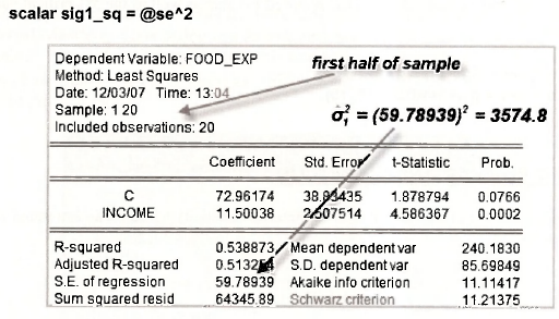
To use the first 20 observations to estimate σ21, we restrict the Sample for estimation as shown below.
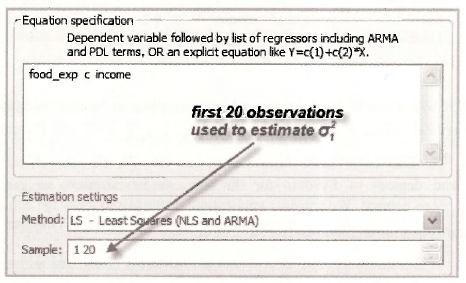
The value σ21 is obtained by squaring the value of S.E. of regression in the resulting output. We give it the name SIG1_SQ.
A similar exercise is followed for the second half of the sample.
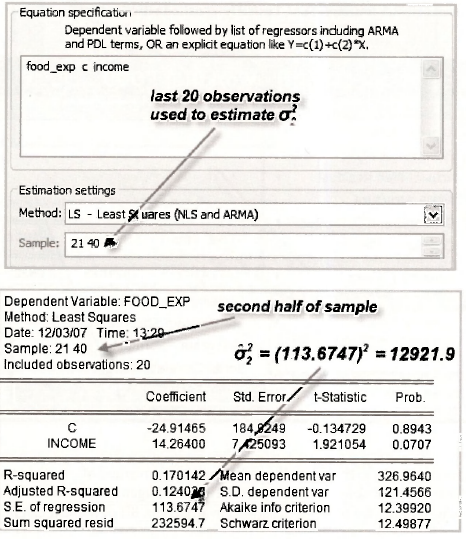
scalar sig2_sq = @seˆ2
Then, the following two commands yield the required E-value as well as the 5% critical value to compare it against.
scalar f_val = sig2_sq/sig1_sq
scalar fcrit = @qfdist(0.95,18,18)
7. TESTING THE VARIANCE FUNCTION
There are a large number of alternative tests for heteroskedasticity based on an estimated variance function of the form
![]()
where e2 are the squared least-squares residuals and z2,z3,…,zs are the variance equation regressors. EViews has the capability to automatically compute test statistic values for these tests as well as their corresponding /7-values. To locate this facility open the least-squares estimated equation and then select View/Residual Tests/Heteroskedasticity Tests.
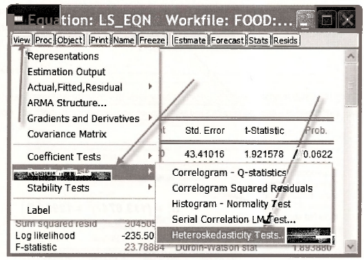
A large number of possibilities – more than you have ever dreamed of – will appear. In line with p. 215 of the text, we will consider just two, the Breusch-Pagan test and the White test. We will also indicate where values for the tests described in Appendix 8B of the text can be found.
7.1. The Breusch-Pagan test
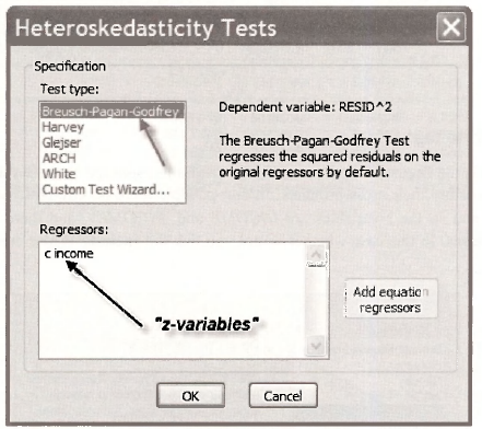
The Breusch-Pagan test (also called Breusch-Pagan-Godfrey test to recognize that Godfrey independently derived the test at about the same time as Breusch and Pagan) can be selected from the Heteroskedasticity Tests dialog box as indicated below. You have the option of selecting the “z-variables”. If you do nothing, EViews will automatically insert those in the mean regression equation. For future reference, inserting INCOME and INCOME2 leads to the White test example of the next section.
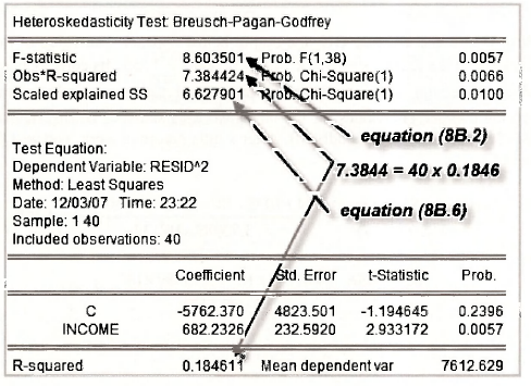
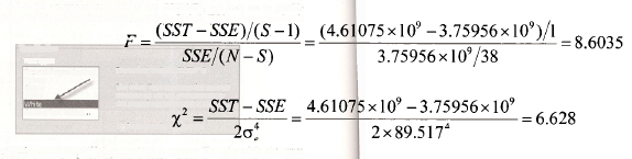
The value of the chi-square statistic considered in the text is x– = N x R2 = 40 x 0.1846 = 7.38. Its corresponding p-value is 0.0066, leading to rejection of H0 at a 5% significance level. The above screen shot shows where these values can be located on the output. There are also values for another two tests statistics on this output. If you are curious about where these values come from, read Appendix 8B. Using equations (8B.2) and (8B.6), you will discover
7.2. The White test
The White test is the Breusch-Pagan test with the z-variables selected as the x-variables and their squares, and possibly their cross-products. In our example there is only one x-variable, namely x = INCOME and so the z-variables are INCOME and INCOME2, and there are no possible cross product terms. In this case whether or not you tick the Include White cross terms box is irrelevant.
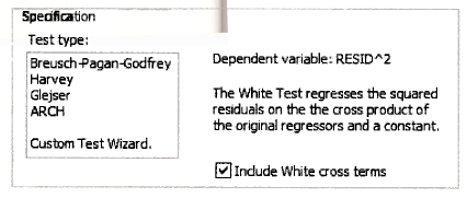
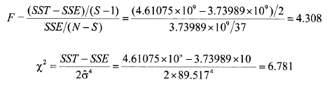
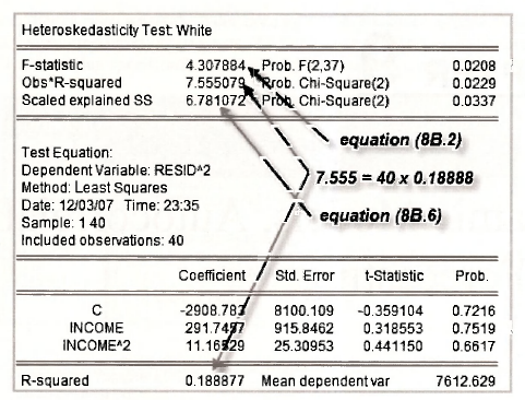
After selecting White and clicking OK, the output below appears. The value of the chi-square statistic considered in the text is x = N x R2 = 40 x 0.18888 = 7.555 . Its corresponding p-value is 0.0229, leading to rejection of H0 at a 5% significance level. Can you see where these values can be located on the output? The values for the other two tests statistics on this output come from equations (8B.2) and (8B.6) in Appendix 8B. After a little detective work, you will discover they are calculated as
Source: Griffiths William E., Hill R. Carter, Lim Mark Andrew (2008), Using EViews for Principles of Econometrics, John Wiley & Sons; 3rd Edition.
20 Sep 2021
20 Sep 2021
20 Sep 2021
20 Sep 2021
20 Sep 2021
20 Sep 2021