1. POLYNOMIALS
In microeconomics you studied “cost” curves and “product” curves that describe a firm. Total cost and total product curves are mirror images of each other, taking the standard “cubic” shapes shown in POE Figure 7.1. Average and marginal cost curves, and their mirror images, average and marginal product curves, take quadratic shapes, usually represented as shown in POE Figure 7.2. The slopes of these relationships are not constant and cannot be represented by regression models that are “linear in the variables.” However, these shapes are easily represented by polynomials. For example, if we consider the average cost relationship a suitable regression model is:
![]()
This quadratic function can take the “U” shape we associate with average cost functions.
To illustrate we use a wage equation with wages a function of education and the worker’s years of experience. What we expect is that young, inexperienced workers will have relatively low wages; with additional experience their wages will rise, but the wages will begin to decline after middle age, as the worker nears retirement. To capture this life-cycle pattern of wages we introduce experience and experience squared to explain the level of wages
![]()
To obtain the inverted-U shape, we expect β3 > 0 and β4 < 0.
In EViews open the workfile cps_smaU.wfl. Save it under a new name, wagechap07.wfl. To estimate the wage equation with quadratic experience we enter the command
![]()
This leads to the estimates
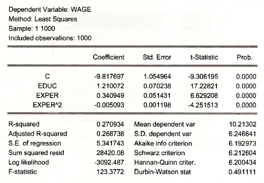
Interpretation in a model that is nonlinear in the variables requires some work. The effect of EDUC on expected WAGE is given by the coefficient 1.21. Each additional year of education is estimated to increase hourly wage by $ 1.21, holding all else constant.
For experience, we must make use of POE equation (7.6). The marginal effect of experience on wage, holding education and other factors constant, is
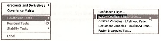
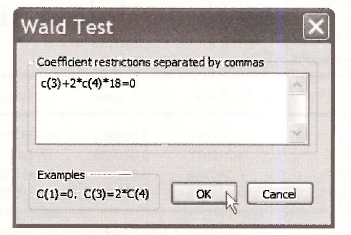
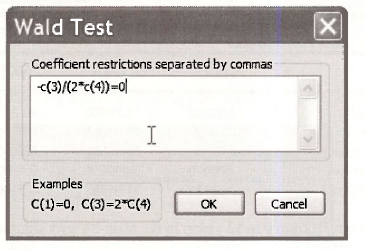
We can evaluate this marginal effect at a particular level of EXPER, such as EXPER = 18. To do this in EViews, from within the regression (which we named WAGE_QUADRATIC) window, select View/Coefficient Tests/Wald-Coefficient Restrictions
Then
Into the test dialog box enter the equation for the marginal effect of experience
Recall that EViews saves the most recent regression results in the coefficient vector called C, and denoted in the EViews workfile by the object
![]()
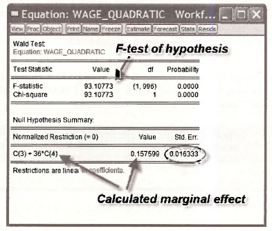
Thus C(3) = b3 and C(4) = b4. The Coefficient restriction we have entered is the marginal effect set equal to zero. This command will not only test the hypothesis that the marginal effect is zero, but it also computes the marginal effect and also computes the standard error of the marginal effect so that interval estimates can easily be created.
It may be useful to have a “picture” of the effect of experience on wage. Open a Group consisting of the variables EDUC, EXPER and WAGE. Do this by holding the Ctrl-key and clicking the series. Then double-click in the blue area. From the spreadsheet, click View/Descriptive Stats/Common Table
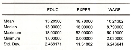
Note that experience ranges from 0 to 52 years. In the main EViews window click on Sample and in the dialog window enter
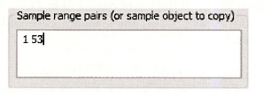
Sample range pairs (or sample object to copy) 153|
Create a series X that will represent years of experience in a plot,
series x = @trend
Using the estimated regression coefficients we can calculate the predicted wages of a person with 13 years of education {EDUC = 13 is the median value) and experience X. The command is
![]()
Now graph the series W against the series X. Select from the main menu Quick/Graph. Then in the Graph Options dialog choose XY Line. The result is a nice visual.
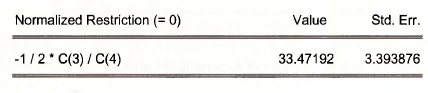
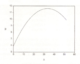 The maximum wage occurs when experience = -p3/2p4. Open the saved regression WAGE QUADRATIC. Select View/Coefficient Tests/Wald-Coefficient Restrictions
This results in the calculation shown at the top of page 170 in POE. We estimate that the turning point in wages occurs at 33.47 years. Using the standard error Std. Err. we can compute an interval estimate if we choose.
Save your workfile and close.
2. DUMMY VARIABLES
Dummy variables are binary 0-1 variables indicating the presence or absence of some condition. Open workfile utown.w/1 containing real estate transaction data from “University Town.”
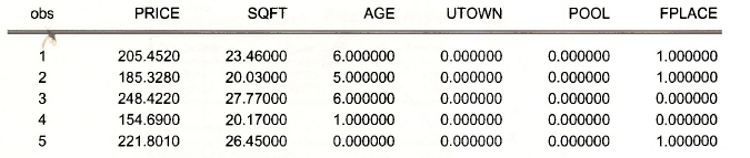
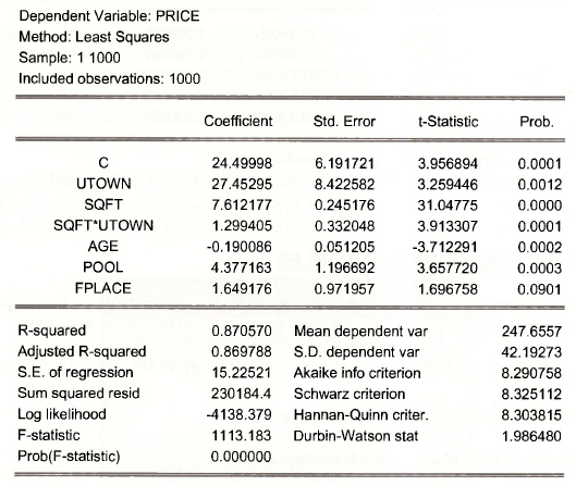
Opening a Group (hold Ctrl click each series, double-click in blue) with the variables we see that PRICE, SQFT and AGE contain the usual type of values, but the rest are 0’s and 1 ’s. These are dummy variables. They are used in a regression just like any other variables. Estimate the POE equation (7.13). Use Quick/Estimate Equation or enter the command
Is price c utown sqft sqft*utown age pool fplace
The result is
2.1. Creating dummy variables
Creating dummy variables is not exactly like creating any other variable. To create a dummy variable that is 1 for large houses, and zero otherwise we must decide what a large house is. The summary statistics for SQFT shows that the median house size in the sample is 2536 square feet. Because SQFT is measured in 100’s of square feet, this is SQFT = 25.36. Suppose that houses larger than this size we take to be “large”. On the workfile window click the Genr button and enter
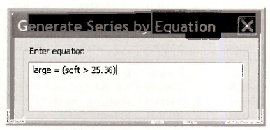
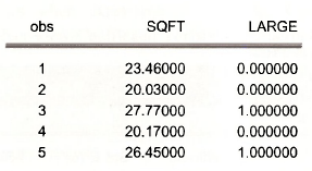
What this does is create a new variable, LARGE, that takes the value 1 if the statement (sqft > 25.36) is true for a particular observation, and zero otherwise. Looking the first few observations we can see that this has worked.
Search for Help on Operators for more information.
Save the workfile as utown_chap07.wfl to maintain the original workfile, and close.
3. INTERACTING DUMMY VARIABLES
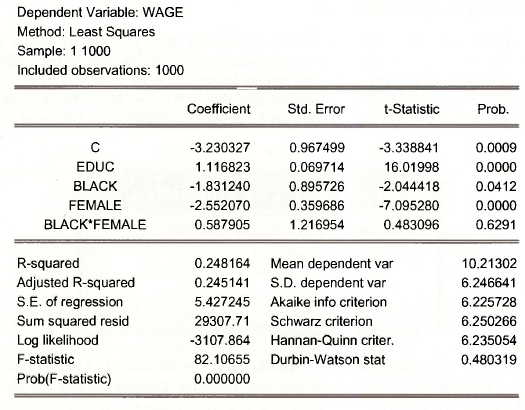
To illustrate further aspects of dummy variables, open cps small.wfl. Save the file under the name cps_small_chap07.wfl. Estimate the wage equation given in POE on page 176.
![]()
Use Quick/Estimate Equation or enter the command
Is wage c educ black female black*female
Save the regression results by naming them WAGE_EQN.
In the regression results window, select View/Representations. The estimation equation is Estimation Equation:
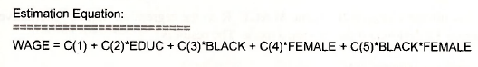
To test the hypothesis that neither race nor gender affects wage we formulate the null hypothesis
![]()
In the regression window, select View/Coefficient TestsAVald – Coefficient Restrictions. Using the equation representation we see that it is the coefficients C(3), C(4) and C(5) that we wish to test.
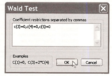
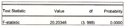
The result is
Alternatively, to directly use the F-statistic,
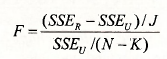
we require the sum of squared least squares residuals from the unrestricted model and the model that is restricted by the null hypothesis. The WAGE regression is the unrestricted model in this case, and the SSEV is
Sum squared resid 29307.71
To obtain the restricted model we omit the variables BLACK, FEMALE and their interaction. Use the command
equation wage_r.ls wage c educ
Recall that this notation assigns the name WAGE_R to the regression object. Alternatively use Quick/Estimate Equation and then assign a name. The result is
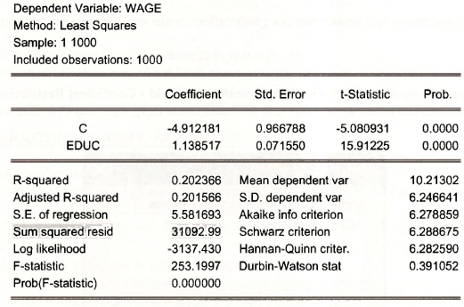
The “restricted” sum of squared residuals is SSEr = 31092.99. Using these values the F = 20.20 can be calculated.
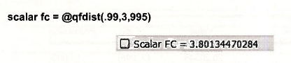
The critical value for the test comes from an F-distribution with 3 numerator degrees of freedom and 995 denominator degrees of freedom. The critical value is computed using @qfdist.
4. DUMMY VARIABLES WITH SEVERAL CATEGORIES
Open cps smalLwfl. Save the fde as wage_regions_chap07.wfl. Estimate the regression shown in Table 7.5 on POE page 178. On the command line enter
equation regions.Is wage c educ black black*female south midwest west
The result is on the next page.
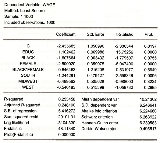
Select View/Representations in the regression window. We see that the estimation equation is Estimation Equation:

Test the null hypothesis that there are no regional differences by selecting View/Coefficient Tests/Wald – Coefficient Restrictions.
Enter the null hypothesis that coefficients 6, 7 and 8 are zero.
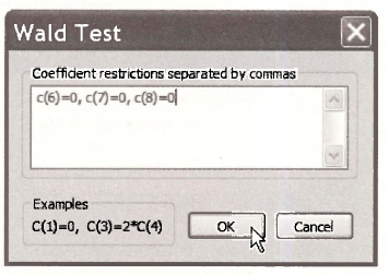
The result is
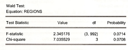
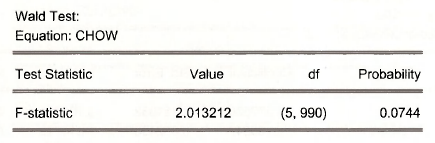
The F-statistic’s p-value shows that we reject the null hypothesis of no regional differences at the 10% level of significance, but not at the 5% level. The Chi-square statistic is an alternative approach to the test.
To construct the F-statistic directly we need the “unrestricted” sum of squared residuals in REGIONS model above. The “restricted” sum of squared errors comes from the model omitting the regional dummies. We obtained this result in Section 7.3. But it is easy to replicate them using
equation regions_rest.ls wage c educ black female black*female
5. TESTING THE EQUIVALENCE OF TWO REGRESSIONS
The Chow test is illustrated using cps small.wfl in Section 7.3.3 of POE. The WAGE model in POE equation (7.16) is obtained by interacting the variable SOUTH with the variables EDUC, BLACK, FEMALE and BLACK * FEMALE
The estimation can be carried out using the command
Is wage c educ black female black*female south educ*south black*south female*south black*female*south
The result is shown on the next page.
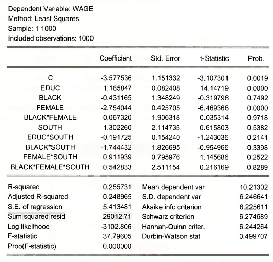
Select View/Representations to see the estimation equation Estimation Equation:
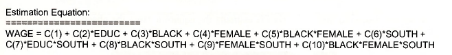
To test the null hypothesis that wages for the SOUTH are no different from the rest of the country we test that coefficients 6-10 are zero.
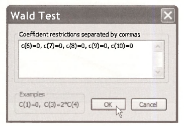
The F-test statistic value is
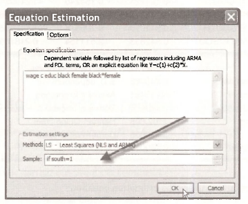
Obtaining the regression for the SOUTH observations is obtained by selecting Quick/Estimate Equation. In the dialog box enter the equation and modify the Sample to include observations for which SOUTH = 1.
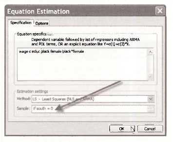
To obtain the results for the NONSOUTH estimate the equation using the observations for which SOUTH = 0.
6. INTERACTIONS BETWEEN CONTINUOUS VARIABLES
Open the workfile pizza.wfl. Estimate the least squares regression of PIZZA on AGE and INCOME.
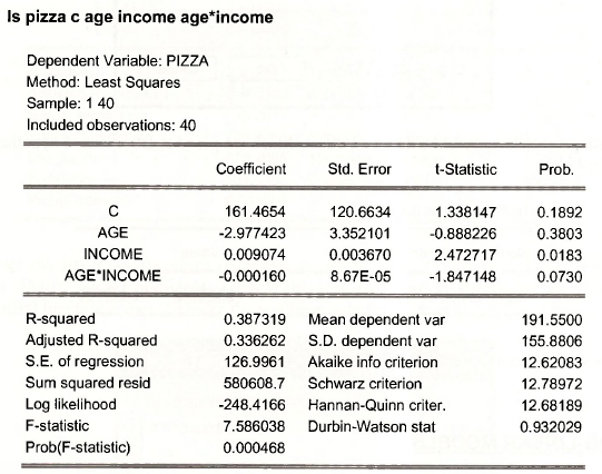
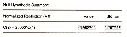
The marginal effect of AGE is
![]()
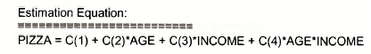
To evaluate this marginal effect at INCOME = $25,000, select in the regression window View/Repesentations to see
Then select View/Coefficient Tests/Wald – Coefficient Restrictions.
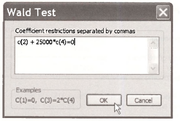
The Wald test results include the marginal effect, which we posed to EViews as a hypothesis, and its standard error.
Save this workfile and close.
7. LOG-LINEAR MODELS
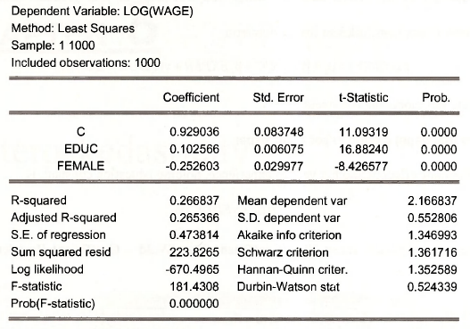
Regression equations with log-transformed dependent variables are common. To illustrate, open the workfile cps smd.ll.wfl. In EViews the function log creates the natural logarithm. The estimation equation can be represented as
Is log(wage) c educ female
The result (next page) is as shown on page 185 of POE.
The exact calculation of the effect of gender on wages looks complicated, but it is simple in EViews. Select View/Coefficient Tests/Wald – Coefficient Restrictions. In EViews the exponential function is exp. To make the nonlinear calculation enter it as a hypothesis.
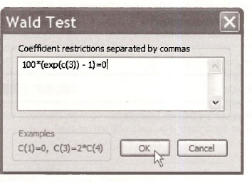
The result is
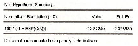
The calculated percentage difference in wages is -22.32% and EViews computes a standard error for this quantity by the “Delta method,” which you will study in your graduate econometrics courses.
The next example includes an interaction term
![]()
To estimate this model the command is
Is log(wage) c educ exper educ*exper
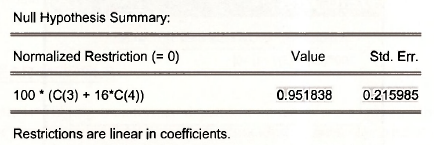
The approximate effect of another year of experience, holding education constant, is
![]()
Using the same approach, select View/Coefficient Tests/Wald – Coefficient Restrictions and enter
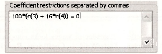
This yields the estimated benefit of another year of experience, 0.95%.
Source: Griffiths William E., Hill R. Carter, Lim Mark Andrew (2008), Using EViews for Principles of Econometrics, John Wiley & Sons; 3rd Edition.
20 Sep 2021
27 Oct 2020
20 Sep 2021
20 Sep 2021
20 Sep 2021
20 Sep 2021