Problem 4.5: Frequency Tables for a Few Variables with SPSS

Displaying Frequency tables for variables can help you understand how many participants are in each level of a variable and how much missing data of various types you have. For nominal variables, most descriptive statistics are meaningless. Thus, having a frequency table is usually the best way to understand your nominal variables. We created a frequency table for the nominal variable religion in Chapter 3 so we will not redo it here.

4.5. Examine the data to get a good understanding of the frequencies of scores for one nominal variable plus one scale/normal, one ordinal, and one dichotomous variable.

Use the following commands:

• Select Analyze → Descriptive Statistics → Frequencies.
• Click on Reset if any variables are in the Variable(s)
• Now highlight the nominal variable ethnicity in the left box.
• Click on the arrow button pointing right.
• Highlight and move over one scale variable (we chose visualization retest), one ordinal variable (we chose father’s education), and one dichotomous variable (we used gender).
• Be sure the Display frequency tables box is checked.
• Do not click on Statistics because we do not want to select any this time.
• Click on OK

Compare your output to Output 4.5. If it looks the same, you have done the steps correctly.

Output 4.5 Frequency Tables for Four Variables

FREQUENCIES VARIABLES=ethnic visual2 faed gend /ORDER= ANALYSIS .

Frequencies

Interpretation of Output 4.5

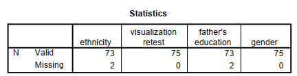
The first table, entitled Statistics, provides, in this case, only the number of participants for whom we have Valid data and the number with Missing data. We did not request any other statistics because almost all of them (e.g., skewness, standard deviation) are not appropriate to use with the nominal and dichotomous data, and we have such statistics for the ordinal and normal/scale variables.

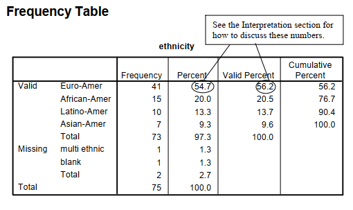
The other four tables are labeled Frequency Table; there is one for ethnicity, one for visualization test, one for father’s education, and one for gender. The left-hand column shows the Valid categories (or levels or values), Missing values, and Total number of participants. The Frequency column gives the number of participants who had each value. The Percent column is the percent who had each value, including missing values. For example, in the ethnicity table, 54.7% of all participants were Euro-American, 20.0% were African American, 13.3% were Latino-American, and 9.3% were Asian American. There was also a total of 2.7% missing; 1.3% were multiethnic, and 1.3% were left blank. The valid percent shows the percent of those with nonmissing data at each value; for example, 56.2% of the 73 students with a single listed ethnic group were Euro-Americans. Finally, Cumulative Percent is the percent of subjects in a category plus the categories listed above it; however, this is not meaningful for ethnicity unless you want to know the percent of participants who are not Asian American.

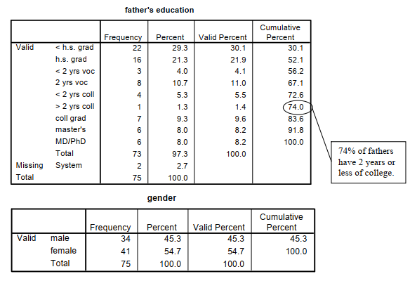
As mentioned in Chapter 3, this last column usually is not very useful with nominal data, but can be quite informative for frequency distributions with several ordered categories. For example, in the distribution of father’s education, 74% of the fathers had less than a bachelor’s degree (i.e., they had not graduated from college).

Source: Morgan George A, Leech Nancy L., Gloeckner Gene W., Barrett Karen C.

(2012), IBM SPSS for Introductory Statistics: Use and Interpretation, Routledge; 5th edition; download Datasets and Materials.