Problem 4.4: Descriptives for Dichotomous Variables with SPSS

Now let’s explore the dichotomous variables. To do this, we do the Descriptives command for each of the dichotomous variables. Once again, we could have done Frequencies, with or without frequency tables, but we chose Descriptives. This time we select fewer statistics because the standard deviation, variance, and skewness values are not very meaningful with dichotomous variables.

4.4. Examine the data to get a good understanding of each of the dichotomous variables.

When using the Descriptives command to compute basic descriptive statistics for the dichotomous variables, you need to do these steps:

• Select Analyze → Descriptive Statistics → Descriptives.

After selecting Descriptives, you will be ready to compute the N, minimum, maximum, and mean for all participants or cases on all selected variables in order to examine the data.

• Before starting this problem, press Reset (see Fig. 4.1) to clear the Variable
• While holding down the control key (i.e., “Ctrl”) highlight all of the dichotomous variables in the left box. These variables have only two levels. They are: gender, algebra 1, algebra 2, geometry, trigonometry, calculus, and math grades.
• Click on the arrow button pointing right.
• Be sure that all of these variables have moved out of the left window and into the Variable(s) window.
• Click on The Descriptives: Options window will open.
• Select Mean, Minimum, and Maximum.
• Unclick Deviation.
• Click on
• Click on OK.

Compare your output to Output 4.4. If it looks the same, you have done the steps correctly.

Output 4.4: Descriptives for Dichotomous Variables

DESCRIPTIVES VARIABLES=gender alg1 alg2 geo trig calc mathgr /STATISTICS= MEAN MIN MAX .

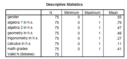
Descriptives

Interpretation of Output 4.4

Output 4.4 includes only one table of Descriptive Statistics. Across the top row are the requested statistics of N, Minimum, Maximum, and Mean. We could have requested other statistics, but they would not be very meaningful for dichotomous variables. Down the left column are the variable labels. The N column indicates that all the variables have complete data. The Valid N (listwise) is 75, which also indicates that all the participants had data for each of our requested variables.

The most helpful column is the Mean column. Although the mean is not meaningful for nominal variables with more than two categories, you can use the mean of dichotomous variables to understand what percentage of participants fall into each of the two groups. For example, the mean of gender is .55, which indicates that that 55% of the participants were coded as 1 (female); thus 45% were coded 0 (male). Because the mean is greater than .50, there are more females than males. If the mean is close to 1 or 0 (see algebra 1 and calculus), then splitting the data on that dichotomous variable might not be useful because there will be many participants in one group and very few participants in the other.

Checking for errors. The Minimum column shows that all the dichotomous variables had “0” for a minimum and the Maximum column indicates that all the variables have “1” for a maximum. This is good because it agrees with the codebook.

Source: Morgan George A, Leech Nancy L., Gloeckner Gene W., Barrett Karen C.

(2012), IBM SPSS for Introductory Statistics: Use and Interpretation, Routledge; 5th edition; download Datasets and Materials.