Some Alternative Theories of Portfolio Theory and the Capital Asset Pricing Model

The capital asset pricing model pictures investors as solely concerned with the level and uncertainty of their future wealth. But this could be too simplistic. For example, investors may become accustomed to a particular standard of living, so that poverty tomorrow may be particularly difficult to bear if you were wealthy yesterday. Behavioral psychologists have also observed that investors do not focus solely on the current value of their holdings, but look back at whether their investments are showing a profit. A gain, however small, may be an additional source of satisfaction. The capital asset pricing model does not allow for the possibility that investors may take account of the price at which they purchased stock and feel elated when their investment is in the black and depressed when it is in the red.

1. Arbitrage Pricing Theory

The capital asset pricing theory begins with an analysis of how investors construct efficient portfolios. Stephen Ross’s arbitrage pricing theory, or APT, comes from a different family entirely. It does not ask which portfolios are efficient. Instead, it starts by assuming that each stock’s return depends partly on pervasive macroeconomic influences or “factors” and partly on “noise”—events that are unique to that company. Moreover, the return is assumed to obey the following simple relationship:

The theory does not say what the factors are: There could be an oil price factor, an interest- rate factor, and so on. The return on the market portfolio might serve as one factor, but then again it might not.

Some stocks will be more sensitive to a particular factor than other stocks. ExxonMobil would be more sensitive to an oil price factor than, say, Coca-Cola. If factor 1 picks up unex­pected changes in oil prices, b1 will be higher for ExxonMobil.

For any individual stock, there are two sources of risk. First is the risk that stems from the pervasive macroeconomic factors. This cannot be eliminated by diversification. Second is the risk arising from possible events that are specific to the company. Diversification eliminates specific risk, and diversified investors can therefore ignore it when deciding whether to buy or sell a stock. The expected risk premium on a stock is affected by factor or macroeconomic risk; it is not affected by specific risk.

Arbitrage pricing theory states that the expected risk premium on a stock should depend on the expected risk premium associated with each factor and the stock’s sensitivity to each of the factors (b₁₍ b₂, b₃, etc.). Thus the formula is

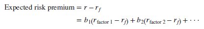
Notice that this formula makes two statements:

1. If you plug in a value of zero for each of the b’s in the formula, the expected risk premium is zero. A diversified portfolio that is constructed to have zero sensitivity to each macroeconomic factor is essentially risk-free and therefore must be priced to offer the risk-free rate of interest. If the portfolio offered a higher return, investors could make a risk-free (or “arbitrage”) profit by borrowing to buy the portfolio. If it offered a lower return, you could make an arbitrage profit by running the strategy in reverse; in other words, you would sell the diversified zero-sensitivity portfolio and invest the proceeds in U.S. Treasury bills.

2. A diversified portfolio that is constructed to have exposure to, say, factor 1, will offer a risk premium, which will vary in direct proportion to the portfolio’s sensitivity to that factor. For example, imagine that you construct two portfolios, A and B, that are affected only by factor 1. If portfolio A is twice as sensitive as portfolio B to factor 1, portfolio A must offer twice the risk premium. Therefore, if you divided your money equally between U.S. Treasury bills and portfolio A, your combined portfolio would have exactly the same sensitivity to factor 1 as portfolio B and would offer the same risk premium.

Suppose that the arbitrage pricing formula did not hold. For example, suppose that the combination of Treasury bills and portfolio A offered a higher return. In that case investors could make an arbitrage profit by selling portfolio B and investing the proceeds in the mixture of bills and portfolio A.

The arbitrage that we have described applies to well-diversified portfolios, where the specific risk has been diversified away. But if the arbitrage pricing relationship holds for all diversified portfolios, it must generally hold for the individual stocks. Each stock must offer an expected return commensurate with its contribution to portfolio risk. In the APT, this contribution depends on the sensitivity of the stock’s return to unexpected changes in the macroeconomic factors.

2. A Comparison of the Capital Asset Pricing Model and Arbitrage Pricing Theory

Like the capital asset pricing model, arbitrage pricing theory stresses that expected return depends on the risk stemming from economywide influences and is not affected by specific risk. You can think of the factors in arbitrage pricing as representing special portfolios of stocks that tend to be subject to a common influence. If the expected risk premium on each of these portfolios is proportional to the portfolio’s market beta, then the arbitrage pricing theory and the capital asset pricing model will give the same answer. In any other case, they will not.

How do the two theories stack up? Arbitrage pricing has some attractive features. For example, the market portfolio that plays such a central role in the capital asset pricing model does not feature in arbitrage pricing theory.^[3] So we do not have to worry about the problem of measuring the market portfolio, and in principle we can test the arbitrage pricing theory even if we have data on only a sample of risky assets.

Unfortunately, you win some and lose some. Arbitrage pricing theory does not tell us what the underlying factors are—unlike the capital asset pricing model, which collapses all macroeconomic risks into a well-defined single factor, the return on the market portfolio.

3. The Three-Factor Model

Look back at the equation for APT. To estimate expected returns, you first need to follow three steps:

Step 1: Identify a reasonably short list of macroeconomic factors that could affect stock returns.

Step 2: Estimate the expected risk premium on each of these factors (r_factor 1 – f etc.).

Step 3: Measure the sensitivity of each stock to the factors (bj, b₂, etc.).

One way to shortcut this process is to take advantage of the research by Fama and French, which showed that stocks of small firms and those with a high book-to-market ratio have provided above-average returns. This could simply be a coincidence. But there is also some evidence that these factors are related to company profitability and therefore may be picking up risk factors that are left out of the simple CAPM.^[4]

If investors do demand an extra return for taking on exposure to these factors, then we have a measure of the expected return that looks very much like arbitrage pricing theory:

This is commonly known as the Fama-French three-factor model. Using it to estimate expected returns is the same as applying the arbitrage pricing theory. Here is an example

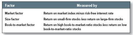
Step 1: Identify the Factors Fama and French have already identified the three factors that appear to determine expected returns. The returns on each of these factors are

Step 2: Estimate the Risk Premium for Each Factor We will keep to our figure of 7% for the market risk premium. History may provide a guide to the risk premium for the other two fac­tors. As we saw earlier, between 1926 and 2017, the difference between the annual returns on small and large capitalization stocks averaged 3.2% a year, while the difference between the returns on stocks with high and low book-to-market ratios averaged 4.9%.

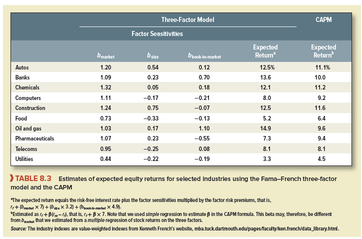
Step 3: Estimate the Factor Sensitivities Some stocks are more sensitive than others to fluc­tuations in the returns on the three factors. You can see this from the first three columns of numbers in Table 8.3, which show some estimates of the factor sensitivities of 10 indus­try groups for the 60 months ending in December 2017. For example, an increase of 1% in the return on the book-to-market factor reduces the return on computer stocks by .21% but increases the return on oil and gas stocks by 1.10%. In other words, when value stocks (high book-to-market) outperform growth stocks (low book-to-market), computer stocks tend to perform relatively badly and oil and gas stocks do relatively well.

Once you have estimated the factor sensitivities, it is a simple matter to multiply each of them by the expected factor return and add up the results. For example, the expected risk pre­mium on pharmaceutical stocks is r – rf = (1.07 X 7) + (.23 X 3.2) – (.55 X 4.9) = 5.5%. To calculate the expected return we need to add on the risk-free interest rate, which we assume to be 1.8%. Thus the three-factor model suggests that expected return on pharmaceutical stocks is 1.8 + 5.5 = 7.3%.

Compare this figure with the expected return estimate using the capital asset pricing model (the final column of Table 8.3). The three-factor model provides a slightly lower estimate of the expected return for pharmaceutical stocks. Why? Largely because they are growth stocks with a low exposure (-.55) to the book-to-market factor. The three-factor model produces a lower expected return for growth stocks, but it produces a higher figure for value stocks such as those of banks and oil companies that have a high book-to-market ratio.

This Fama-French APT model is not widely used in practice to estimate the cost of equity or the WACC. The model requires three betas and three risk premiums, instead of one beta and one market risk premium in the CAPM. Also the three APT betas are not as easy to predict and interpret as the CAPM beta, which is just an exposure to overall market risk. The Fama-French APT is probably less suited to estimating the cost of equity for an indi­vidual stock than to providing an alternative way to estimate an industry cost of equity, as in Table 8.3.

The Fama-French model finds its widest use as a way of measuring the performance of mutual funds, pension funds, and other professionally managed portfolios. If a portfolio man­ager “beats the S&P,” it may be because he or she has made a bet on small stocks in a period when small stocks soared—or perhaps he or she had the luck or foresight to avoid growth stocks in a period when growth stocks collapsed. An analyst can evaluate the manager’s performance by estimating the portfolio’s b_market, b_size, and b_{book-to-market} and then checking whether the portfolio return is better than the return on a robotically managed portfolio with the same exposures to the Fama-French factors.

Source:  Brealey Richard A., Myers Stewart C., Allen Franklin (2020), Principles of Corporate Finance, McGraw-Hill Education; 13th edition.