Almost all real-world investment decisions entail either-or choices. Such choices are said to be mutually exclusive. We came across an example of mutually exclusive investments in Chapter 2. There we looked at whether it was better to build an office block for immediate sale or to rent it out and sell it at the end of two years. To decide between these alternatives, we calculated the NPV of each and chose the one with the higher NPV.
That is the correct procedure as long as the choice between the two projects does not affect any future decisions that you might wish to make. But sometimes the choices that you make today will have an impact on future opportunities. When that is so, choosing between competing projects is trickier. Here are four important, but often challenging, problems:
- The investment timing problem. Should you invest now or wait and think about it again next year? (Here, today’s investment is competing with possible future investments.)
- The choice between long- and short-lived equipment. Should the company save money today by choosing cheaper machinery that will not last as long? (Here, today’s decision would accelerate a later investment in machine replacement.)
- The replacement problem. When should existing machinery be replaced? (Using it another year could delay investment in more modern equipment.)
- The cost of excess capacity. What is the cost of using equipment that is temporarily not being used? (Increasing use of the equipment may bring forward the date at which additional capacity is required.)
We will look at each of these problems in turn.
1. Problem 1: The Investment Timing Decision
The fact that a project has a positive NPV does not mean that it is best undertaken now. It might be even more valuable if undertaken in the future. The question of optimal timing is not difficult when the cash flows are certain. You must first examine alternative start dates (t) for the investment and calculate the net future value at each of these dates. Then, to find which of the alternatives would add most to the firm’s current value, you must discount these net future values back to the present:
For example, suppose you own a large tract of inaccessible timber. To harvest it, you need to invest a substantial amount in access roads and other facilities. The longer you wait, the higher the investment required. On the other hand, lumber prices may rise as you wait, and the trees will keep growing, although at a gradually decreasing rate.
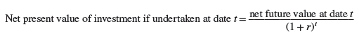
Let us suppose that the net present value of the harvest at different future dates is as follows:
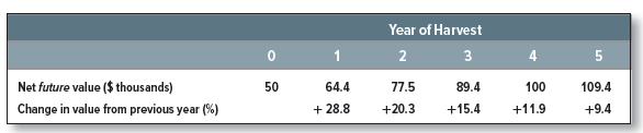
As you can see, the longer you defer cutting the timber, the more money you will make. However, your concern is with the date that maximizes the net present value of your investment, that is, its contribution to the value of your firm today. You therefore need to discount the net future value of the harvest back to the present. Suppose the appropriate discount rate is 10%. Then, if you harvest the timber in year 1, it has a net present value of $58,500:
![]()
The net present value for other harvest dates is as follows:
The optimal point to harvest the timber is year 4 because this is the point that maximizes NPV.
Notice that before year 4, the net future value of the timber increases by more than 10% a year: The gain in value is greater than the cost of the capital tied up in the project. After year 4, the gain in value is still positive but less than the required return. So delaying the harvest further just reduces shareholder wealth.
The investment timing problem is much more complicated when you are unsure about future cash flows. We return to the problem of investment timing under uncertainty in Chapters 10 and 22.
2. Problem 2: The Choice between Long- and Short-Lived Equipment
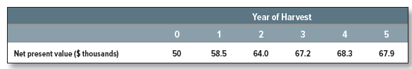
An advertising agency needs to choose between two digital presses. Let’s call them machines A and B. The two machines are designed differently but have identical capacity and do exactly the same job. Machine A costs $15,000 and will last three years. It costs $5,000 per year to run. Machine B is an “economy” model, costing only $10,000, but it will last only two years and costs $6,000 per year to run.
The only way to choose between these two machines is on the basis of cost. The present value of each machine’s cost is as follows:
Should the agency take machine B, the one with the lower present value of costs? Not necessarily. All we have shown is that machine B offers two years of service for a lower total cost than three years of service from machine A. But is the annual cost of using B lower than that of A?
Suppose the financial manager agrees to buy machine A and pay for its operating costs out of her budget. She then charges the annual amount for use of the machine. There will be three equal payments starting in year 1. The financial manager has to make sure that the present value of these payments equals the present value of the costs of each machine.
When the discount rate is 6%, the payment stream with such a present value turns out to be $10,610 a year. In other words, the cost of buying and operating machine A over its three-year life is equivalent to an annual charge of $10,610 a year for three years.
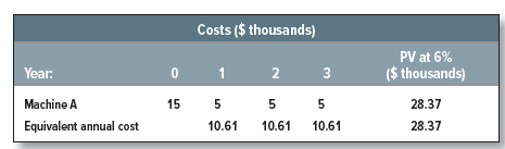
We calculated this equivalent annual cost by finding the three-year annuity with the same present value as A’s lifetime costs.
PV of annuity = PV of A’s costs = 28.37
= annuity payment X 3-year annuity factor
At a 6% cost of capital, the annuity factor is 2.673 for three years, so
![]()
A similar calculation for machine B gives an equivalent annual cost of $11,450:
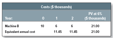
Machine A is better because its equivalent annual cost is less ($10,610 versus $11,450 for machine B).
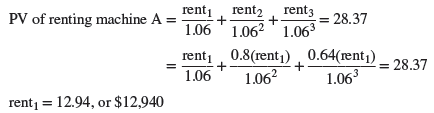
Equivalent Annual Cash Flow, Inflation, and Technological Change When we calculated the equivalent annual costs of machines A and B, we implicitly assumed that inflation is zero. But, in practice, the cost of buying and operating the machines is likely to rise with inflation. If so, the nominal costs of operating the machines will rise, while the real costs will be constant. Therefore, when you compare the equivalent annual costs of two machines, we strongly recommend doing the calculations in real terms. Do not calculate equivalent annual cash flows as level nominal annuities. This procedure can give incorrect rankings of true equivalent annual flows at high inflation rates. See Challenge Problem 37 at the end of this chapter for an example.[1]
There will also be circumstances in which even the real cash flows of buying and operating the two machines are not expected to be constant. For example, suppose that thanks to technological improvements, new machines cost 20% less each year in real terms to buy and operate. In this case, future owners of brand-new, lower-cost machines will be able to cut their (real) rental cost by 20%, and owners of old machines will be forced to match this reduction. Thus, we now need to ask: If the real level of rents declines by 20% a year, how much will it cost to rent each machine?
If the real rent for year 1 is rentj, then the real rent for year 2 is rent2 = 0.8 X rentj. Rent3 is 0.8 X rent2, or 0.64 X rentj. The owner of each machine must set the real rents sufficiently high to recover the present value of the costs. If the real cost of capital is 6%:
For machine B:
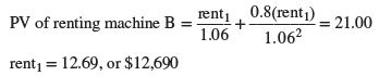
The merits of the two machines are now reversed. Once we recognize that technology is expected to reduce the real costs of new machines, then it pays to buy the shorter-lived machine B rather than become locked into an aging technology with machine A in year 3.
You can imagine other complications. Perhaps machine C will arrive in year 1 with an even lower equivalent annual cost. You would then need to consider scrapping or selling machine B at year 1 (more on this decision follows). The financial manager could not choose between machines A and B in year 0 without taking a detailed look at what each machine could be replaced with.
Comparing equivalent annual cash flows should never be a mechanical exercise; always think about the assumptions that are implicit in the comparison. Finally, remember why equivalent annual cash flows are necessary in the first place. It is because A and B will be replaced at different future dates. The choice between them therefore affects future investment decisions. If subsequent decisions are not affected by the initial choice (e.g., because neither machine will be replaced), then we do not need to take future decisions into account.[2]
Equivalent Annual Cash Flow and Taxes We have not mentioned taxes. But you surely realized that machine A and B’s lifetime costs should be calculated after-tax, recognizing that operating costs are tax-deductible and that capital investment generates depreciation tax shields.
3. Problem 3: When to Replace an Old Machine
Our earlier comparison of machines A and B took the life of each machine as fixed. In practice, the point at which equipment is replaced reflects economics, not physical collapse. We must decide when to replace. The machine will rarely decide for us.
Here is a common problem. You are operating an elderly machine that is expected to produce a net cash inflow of $4,000 in the coming year and $4,000 next year. After that it will give up the ghost. You can replace it now with a new machine, which costs $15,000 but is much more efficient and will provide a cash inflow of $8,000 a year for three years. You want to know whether you should replace your equipment now or wait a year.
We can calculate the NPV of the new machine and also its equivalent annual cash flow— that is, the three-year annuity that has the same net present value:
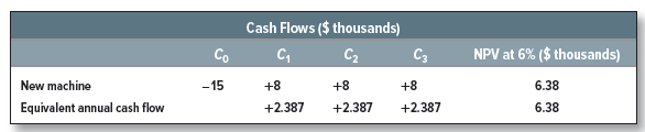
In other words, the cash flows of the new machine are equivalent to an annuity of $2,387 per year. So we can equally well ask at what point we would want to replace our old machine with a new one producing $2,387 a year. When the question is put this way, the answer is obvious. As long as your old machine can generate a cash flow of $4,000 a year, who wants to put in its place a new one that generates only $2,387 a year?
It is a simple matter to incorporate salvage values into this calculation. Suppose that the current salvage value is $8,000 and next year’s value is $7,000. Let us see where you come out next year if you wait and then sell. On one hand, you gain $7,000, but you lose today’s salvage value plus a year’s return on that money. That is 8,000 X 1.06 = $8,480. Your net loss is 8,480 – 7,000 = $1,480, which only partly offsets the operating gain. You should not replace yet.
Remember that the logic of such comparisons requires that the new machine be the best of the available alternatives and that it in turn be replaced at the optimal point.
4. Problem 4: Cost of Excess Capacity
Any firm with a centralized information system (computer servers, storage, software, and telecommunication links) encounters many proposals for using it. Recently installed systems tend to have excess capacity, and since the immediate marginal costs of using them seem to be negligible, management often encourages new uses. Sooner or later, however, the load on a system increases to the point at which management must either terminate the uses it originally encouraged or invest in another system several years earlier than it had planned. Such problems can be avoided if a proper charge is made for the use of spare capacity.
Suppose we have a new investment project that requires heavy use of an existing information system. The effect of adopting the project is to bring the purchase date of a new, more capable system forward from year 4 to year 3. This new system has a life of five years, and at a discount rate of 6%, the present value of the cost of buying and operating it is $500,000.
We begin by converting the $500,000 present value of the cost of the new system to an equivalent annual cost of $118,700 for each of five years.14 Of course, when the new system in turn wears out, we will replace it with another. So we face the prospect of future information- system expenses of $118,700 a year. If we undertake the new project, the series of expenses begins in year 4; if we do not undertake it, the series begins in year 5. The new project, therefore, results in an additional cost of $118,700 in year 4. This has a present value of 118,700/ (1.06)4, or about $94,000. This cost is properly charged against the new project.
When we recognize it, the NPV of the project may prove to be negative. If so, we still need to check whether it is worthwhile undertaking the project now and abandoning it later, when the excess capacity of the present system disappears.
23 Jun 2021
24 Jun 2021
25 Jun 2021
24 Jun 2021
24 Jun 2021
24 Jun 2021