When investigating the difference between two unrelated or independent groups (in this case males and females) on an approximately normal dependent variable, it is appropriate to choose an independent samples t test if the following assumptions are not markedly violated.
Assumptions of the Independent Samples t Test:
- The variances of the dependent variable in the two populations are equal.
- The dependent variable is normally distributed within each population.
- The data are independent (scores of one participant are not related systematically to scores of the others).
SPSS will automatically test Assumption 1 with the Levene’s test for equal variances. Assumption 2 could be tested, as we did in Chapter 4, Problem 4.3, with the Explore command, to see whether the dependent variables are at least approximately normally distributed for each gender. Because the t test is quite robust to violations of this assumption, especially if the data for both groups are skewed in the same direction, we won’t test it here. Assumption 3 probably is met because the genders are not matched or related pairs and there is no reason to believe that one person’s score might have influenced another person’s. This assumption is best addressed during design and data collection. In addition to ensuring that the data meet these assumptions, the researcher should try to ensure that groups or samples are of similar size, as the assumption of homogeneity of variance is most important and more likely to be violated if samples differ markedly in size.
- Do male and female students differ significantly in regard to their average math achievement scores, grades in high school, and visualization test scores?
One feature of this program is that it can do several t tests in a single output if they have the same independent or grouping variable (e.g., gender). In this problem, we computed three separate t tests, one each for math achievement, grades in high school, and visualization test scores; in each males are compared to females.
With more than one dependent variable, one could have chosen to use MANOVA (see Fig. 6.1), especially if these variables were conceptually related and correlated with each other. MANOVA would enable us to see how a linear combination of these three variables was different for boys than for girls. We will not demonstrate MANOVA in this book, but see Leech et al. (in press) IBM SPSS for Intermediate Statistics (4th ed.) for how to compute and interpret MANOVA.
For the t tests, follow these commands:
- Click on Analyze → Compare means → Independent Samples T Test…
- Move math achievement, grades in h.s., and visualization test to the Test (dependent) Variable(s) box and move gender to the Grouping (independent) Variable: box (see Fig. 9.2).
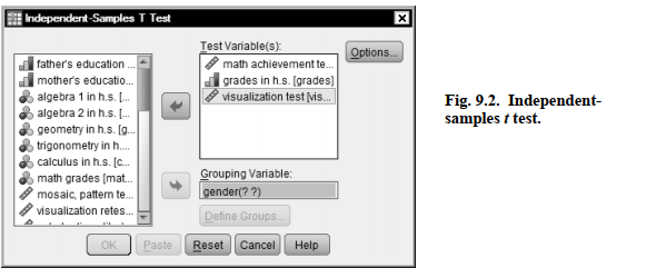
- Next click on Define Groups in Fig. 9.2 to get Fig. 9.3.
- Type 0 (for males) in the Group 1 box and 1 (for females) in the Group 2 box (see Fig. 9.3). This will enable us to compare males and females on each of the three dependent variables.
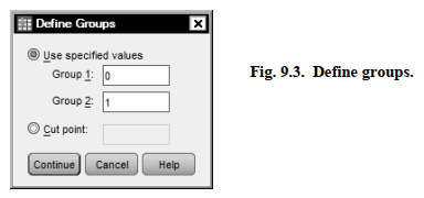
- Click on Continue then on OK. Compare your output to Output 9.2.
Output 9.2: Independent Samples t Test
T-TEST GROUPS=gender(0 1) /MISSING=ANALYSIS
/VARIABLES=mathach grades visual
/CRITERIA=CIN(.95) .
Interpretation of Output 9.2
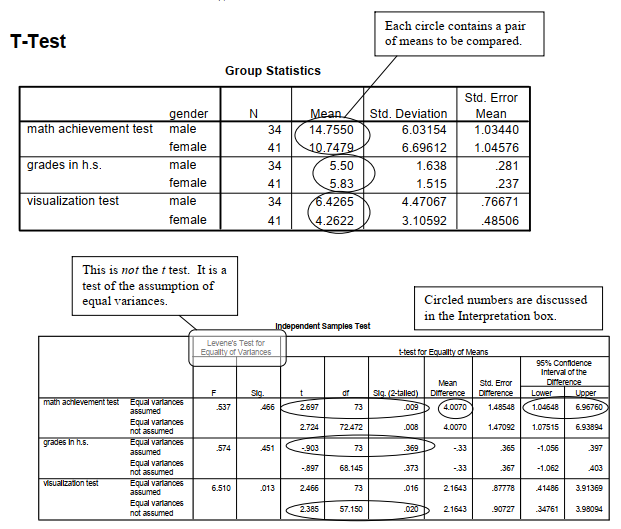
The first table, Group Statistics, shows descriptive statistics for the two groups (males and females) separately. Note that the means within each of the three pairs look somewhat different. This might be due to chance, so we will check the t tests in the next table.
The second table, Independent Samples Test, provides two statistical tests. The left two columns of numbers are the Levene’s test for the assumption that the variances of the two groups are equal. This is not the t test; it only assesses an assumption! If this F test is not significant (as in the case of math achievement and grades in high school), the assumption is not violated, and one uses the Equal variances assumed line for the t test and related statistics. However, if Levene’s F is statistically significant (Sig. < .05), as is true for visualization, then variances are significantly different and the assumption of equal variances is violated. In that case, the Equal variances not assumed line is used, and the t, df, and Sig. are adjusted by the program. The appropriate lines to use are circled in the output.
Thus, for visualization, the appropriate t = 2.39, degrees of freedom (df) = 57.15, and p = .020. This t is statistically significant so, based on examining the means, we can say that boys have higher visualization scores than girls. We used visualization to provide an example where the assumption of equal variances was violated (Levene’s test was significant). Note that for grades in high school, the t is not statistically significant (p = .369) so we conclude that there is no evidence of a systematic difference between boys and girls on grades. On the other hand, for math achievement variances are not significantly different (p = .466) so the assumption is not violated. However, the t is statistically significant because p = .009. Thus, males have higher means.
The 95% Confidence Interval of the Difference is shown in the two right-hand columns of the Output. The confidence interval tells us that if we repeated the study 100 times, 95 of the times the true (population) difference would fall within the confidence interval, which for math achievement is between 1.05 points and 6.97 points. Note that if the Upper and Lower bounds have the same sign (either + and + or – and -), we know that the difference is statistically significant because this means that the null finding of zero difference lies outside of the confidence interval. On the other hand, if zero lies between the upper and lower limits, there could be no difference, as is the case for grades in h.s. The lower limit of the confidence interval on math achievement tells us that the difference between males and females could be as small as 1.05 points out of 25, which is the maximum possible score.
Effect size measures for t tests are not provided in the printout but can be estimated relatively easily. See Chapter 6 for the formula and interpretation of d. For math achievement, the difference between the means (4.01) would be divided by about 6.4, an estimate of the pooled (weighted average) standard deviation. Thus, d would be approximately .60, which is, according to Cohen (1988), a medium to large sized “effect.” Because you need means and standard deviations to compute the effect size, you should include a table with means and standard deviations in your results section for a full interpretation of t tests.
How to Write About Output 9.2.
Results
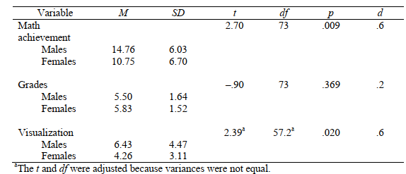
Table 9.2 shows that males were significantly different from females on math achievement (p = .009). Inspection of the two group means indicates that the average math achievement score for female students (M = 10.75) is significantly lower than the score (M = 14.76) for males. The difference between the means is 4.01 points on a 25-point test. The effect size d is approximately .6, which is a typical size for effects in the behavioral sciences. Males did not differ significantly from females on grades in high school (p = .369), but males did score higher on the visualization test (p = .020). The effect size, d, is again approximately .6.
Table 9.2
Comparison of Male and Female High School Students on a Math Achievement Test, Grades, and a Visualization Test (n = 34 males and 41 females)
Source: Morgan George A, Leech Nancy L., Gloeckner Gene W., Barrett Karen C.
(2012), IBM SPSS for Introductory Statistics: Use and Interpretation, Routledge; 5th edition; download Datasets and Materials.
I do agree with all of the ideas you have offered to your post. They are very convincing and can certainly work. Nonetheless, the posts are too short for beginners. Could you please lengthen them a bit from next time? Thank you for the post.