Category: Corporate finance

1. Book Rate of Return

Net present value depends only on the project’s cash flows and the opportunity cost of capital. But when companies report to shareholders, they do not simply show the cash flows. They also report book—that is, accounting—income and book assets.

Financial managers sometimes use these numbers to calculate a book (or accounting) rate of return on a proposed investment. In other words, they look at the prospective book income from the investment as a proportion of the book value of the assets that the firm is proposing to acquire:

They typically compare this figure with the book rate of return that the company is currently earning.

Cash flows and book income are often very different. For example, the accountant labels some cash outflows as capital investments and others as operating expenses. The operating expenses are, of course, deducted immediately from each year’s income. The capital expendi­tures are put on the firm’s balance sheet and then depreciated. The annual depreciation charge is deducted from each year’s income. Thus the book rate of return depends on which items the accountant treats as capital investments and how rapidly they are depreciated.^[1]

Now the merits of an investment project do not depend on how accountants classify the cash flows² and few companies these days make investment decisions just on the basis of the book rate of return. But managers know that the company’s shareholders pay considerable attention to book measures of profitability and naturally they think (and worry) about how major projects would affect the company’s book return. Those projects that would reduce the company’s book return may be scrutinized more carefully by senior management.

You can see the dangers here. The company’s book rate of return may not be a good mea­sure of true profitability. It is also an average across all of the firm’s activities. The average profitability of past investments is not usually the right hurdle for new investments. Think of a firm that has been exceptionally lucky and successful. Say its average book return is 24%, double shareholders’ 12% opportunity cost of capital. Should it demand that all new invest­ments offer 24% or better? Clearly not: That would mean passing up many positive-NPV opportunities with rates of return between 12 and 24%.

We will come back to the book rate of return in Chapters 12 and 28, when we look more closely at accounting measures of financial performance.

2. Payback

We suspect that you have often heard conversations that go something like this: “We are spending $6 a week, or around $300 a year, at the laundromat. If we bought a washing machine for $800, it would pay for itself within three years. That’s well worth it.” You have just encountered the payback rule.

A project’s payback period is found by counting the number of years it takes before the cumulative cash flow equals the initial investment. For the washing machine the payback period was just under three years. The payback rule states that a project should be accepted if its payback period is less than some specified cutoff period. For example, if the cutoff period is four years, the washing machine makes the grade; if the cutoff is two years, it doesn’t.

We have no quarrel with those who use payback as a descriptive statistic. It is perfectly fine to say that the washing machine has a three-year payback. But payback should never be a rule.

Example 5.1 • The Payback Rule

Consider the following three projects:

Project A involves an initial investment of $2,000 (C₀ = -2,000) followed by cash inflows during the next three years. Suppose the opportunity cost of capital is 10%. Then project A has an NPV of +$2,624:

Project B also requires an initial investment of $2,000 but produces a cash inflow of $500 in year 1 and $1,800 in year 2. At a 10% opportunity cost of capital project B has an NPV of -$58:

The third project, C, involves the same initial outlay as the other two projects but its first- period cash flow is larger. It has an NPV of +$50:

The net present value rule tells us to accept projects A and C but to reject project B.

Now look at how rapidly each project pays back its initial investment. With project A, you take three years to recover the $2,000 investment; with projects B and C, you take only two years. If the firm used the payback rule with a cutoff period of two years, it would accept only projects B and C; if it used the payback rule with a cutoff period of three or more years, it would accept all three projects. Therefore, regardless of the choice of cutoff period, the pay­back rule gives different answers from the net present value rule.

You can see why payback can give misleading answers:

1. The payback rule ignores all cash flows after the cutoff date. If the cutoff date is two years, the payback rule rejects project A regardless of the size of the cash inflow in year 3.
2. The payback rule gives equal weight to all cash flows before the cutoff date. The payback rule says that projects B and C are equally attractive, but because C’s cash inflows occur earlier, C has the higher net present value at any positive discount rate.

To use the payback rule, a firm must decide on an appropriate cutoff date. If it uses the same cutoff regardless of project life, it will tend to accept many poor short-lived projects and reject many good long-lived ones.

We have had little good to say about payback. So why do many companies continue to use it? Senior managers don’t truly believe that all cash flows after the payback period are irrelevant. We suggest three explanations. First, payback may be used because it is the simplest way to communicate an idea of project profitability. Investment decisions require discussion and negotiation among people from all parts of the firm, and it is important to have a measure that everyone can understand. Second, managers of larger corporations may opt for projects with short paybacks because they believe that quicker profits mean quicker promotion. That takes us back to Chapter 1, where we discussed the need to align the objec­tives of managers with those of shareholders. Finally, owners of small public firms with limited access to capital may worry about their future ability to raise capital. These worries may lead them to favor rapid payback projects even though a longer-term venture may have a higher NPV.

3. Discounted Payback

Occasionally companies discount the cash flows before they compute the payback period. The discounted cash flows for our three projects are as follows:

The discounted payback measure asks, How many years does the project have to last in order for it to make sense in terms of net present value? You can see that the value of the cash inflows from project B never exceeds the initial outlay and would always be rejected under the discounted payback rule. Thus a discounted payback rule will never accept a negative-NPV project. On the other hand, it still takes no account of cash flows after the cutoff date, so that good long-term projects such as A continue to risk rejection.

Rather than automatically rejecting any project with a long discounted payback period, many managers simply use the measure as a warning signal. These managers don’t unthink­ingly reject a project with a long discounted payback period. Instead they check that the pro­poser is not unduly optimistic about the project’s ability to generate cash flows into the distant future. They satisfy themselves that the equipment has a long life and that competitors will not enter the market and eat into the project’s cash flows.

Source:  Brealey Richard A., Myers Stewart C., Allen Franklin (2020), Principles of Corporate Finance, McGraw-Hill Education; 13th edition.

Whereas payback and return on book are ad hoc measures, internal rate of return has a much more respectable ancestry and is recommended in many finance texts. If we dwell more on its deficiencies, it is not because they are more numerous but because they are less obvious.

In Chapter 2, we noted that the net present value rule could also be expressed in terms of rate of return, which would lead to the following rule: “Accept investment opportunities offer­ing rates of return in excess of their opportunity costs of capital.” That statement, properly interpreted, is absolutely correct. However, interpretation is not always easy for long-lived investment projects.

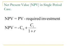
There is no ambiguity in defining the true rate of return of an investment that generates a single payoff after one period:

Alternatively, we could write down the NPV of the investment and find the discount rate that makes NPV = 0.

Of course C₁ is the payoff and -C₀ is the required investment, and so our two equations say exactly the same thing. The discount rate that makes NPV = 0 is also the rate of return.

How do we calculate return when the project produces cash flows in several periods? Answer: We use the same definition that we just developed for one-period projects—the proj­ect rate of return is the discount rate that gives a zero NPV. This discount rate is known as the discounted cash flow (DCF) rate of return or internal rate of return (IRR). The internal rate of return is used frequently in finance. It can be a handy measure, but, as we shall see, it can also be a misleading measure. You should, therefore, know how to calculate it and how to use it properly.

1. Calculating the IRR

The internal rate of return is defined as the rate of discount that makes NPV = 0. So to find the IRR for an investment project lasting T years, we must solve for IRR in the following expression:

Actual calculation of IRR usually involves trial and error. For example, consider a project that produces the following flows:

The internal rate of return is IRR in the equation

Let us arbitrarily try a zero discount rate. In this case, NPV is not zero but +$2,000:

The NPV is positive; therefore, the IRR must be greater than zero. The next step might be to try a discount rate of 50%. In this case, net present value is -$889:

The NPV is negative; therefore, the IRR must be less than 50%. In Figure 5.3, we have plotted the net present values implied by a range of discount rates. From this, we can see that a dis­count rate of 28.08% gives the desired net present value of zero. Therefore, IRR is 28.08%.

(We carry the IRR calculation to two decimal places to avoid confusion from rounding. In practice, no one would worry about the .08%.)^[2]

You can always find the IRR by plotting an NPV profile, as in Figure 5.3, but it is quicker and more accurate to let a spreadsheet or specially programmed calculator do the trial and error for you. The Useful Spreadsheet Functions box near the end of the chapter shows how to use the Excel function to calculate an IRR.

Some people confuse the internal rate of return and the opportunity cost of capital because both appear as discount rates in the NPV formula. The internal rate of return is a profitabil­ity measure that depends solely on the amount and timing of the project cash flows. The opportunity cost of capital is a standard of profitability that we use to calculate how much the project is worth. The opportunity cost of capital is established in the financial markets. It is the expected rate of return offered by other assets with the same risk as the project being evaluated.

2. The IRR Rule

The internal rate of return rule states that the firm should accept an investment project if the opportunity cost of capital is less than the internal rate of return. You can see the reasoning behind this idea if you look again at Figure 5.3. If the opportunity cost of capital is less than the 28.08% IRR, then the project has a positive NPV when discounted at the opportunity cost of capital. If it is equal to the IRR, the project has a zero NPV. And if it is greater than the IRR, the project has a negative NPV. Therefore, when we compare the opportunity cost of capital with the IRR on our project, we are effectively asking whether our project has a positive NPV. This is true not only for our example. The rule will give the same answer as the net present value rule whenever the NPV of a project is a steadily declining function of the discount rate.

The 28.08% internal rate of return on our project tells us how high the opportunity cost of capital must be before the project should be rejected. Although we might not be able to put a precise num­ber on the project’s cost of capital, we might nevertheless be confident that it was less than 28.08% and that we can safely go ahead with the project. You can understand, therefore, why a manager may find it helpful to know the project’s IRR. Our worries concern those managers who use the internal rate of return as a criterion in preference to net present value. Although, properly stated, the two criteria are formally equivalent, the internal rate of return rule contains several pitfalls.

3. Pitfall 1—Lending or Borrowing?

Not all cash-flow streams have NPVs that decline as the discount rate increases. Consider the following projects A and B:

Each project has an IRR of 50%. (In other words, -1,000 + 1,500/1.50 = 0 and +1,000 – 1,500/1.50 = 0.)

Does this mean that they are equally attractive? Clearly not, for in the case of A, where we are initially paying out $1,000, we are lending money at 50%; in the case of B, where we are initially receiving $1,000, we are borrowing money at 50%. When we lend money, we want a high rate of return; when we borrow money, we want a low rate of return.

If you plot a graph like Figure 5.3 for project B, you will find that NPV increases as the discount rate increases. Obviously the internal rate of return rule, as we stated it above, won’t work in this case; we have to look for an IRR less than the opportunity cost of capital.

4. Pitfall 2—Multiple Rates of Return

Helmsley Iron is proposing to develop a new strip mine in Western Australia. The mine involves an initial investment of A$30 billion and is expected to produce a cash inflow of A$10 billion a year for the next nine years. At the end of that time, the company will incur A$65 billion of cleanup costs. Thus, the cash flows from the project are:

Helmsley calculates the project’s IRR and its NPV as follows:

Note that there are two discount rates that make NPV = 0. That is, each of the following state­ments holds:

In other words, the investment has an IRR of both 3.50% and 19.54%. Figure 5.4 shows how this comes about. As the discount rate increases, NPV initially rises and then declines. The reason for this is the double change in the sign of the cash-flow stream. There can be as many internal rates of return for a project as there are changes in the sign of the cash flows.⁴

Decommissioning and clean-up costs can sometimes lead to huge negative cash flows at the end of a project. The cost of decommissioning oil platforms in the British North Sea has been estimated at $75 billion. It can cost more than $500 million to decommission a nuclear power plant. These are obvious instances where cash flows go from positive to negative, but you can probably think of a number of other cases where the company needs to plan for later expenditures. Ships periodically need to go into dry dock for a refit, hotels may receive a major face-lift, machine parts may need replacement, and so on.

Whenever the cash-flow stream is expected to change sign more than once, the company typically sees more than one IRR.

As if this is not difficult enough, there are also cases in which no internal rate of return exists. For example, project C has a positive net present value at all discount rates:

A number of adaptations of the IRR rule have been devised for such cases. Not only are they inadequate, but they also are unnecessary, for the simple solution is to use net present value.

5. Pitfall 3—Mutually Exclusive Projects

Firms often have to choose between several alternative ways of doing the same job or using the same facility. In other words, they need to choose between mutually exclusive projects. Here, too, the IRR rule can be misleading.

Consider projects D and E:

Perhaps project D is a manually controlled machine tool and project E is the same tool with the addition of computer control. Both are good investments, but E has the higher NPV and is, therefore, better. However, the IRR rule seems to indicate that if you have to choose, you should go for D because it has the higher IRR. If you follow the IRR rule, you have the satis­faction of earning a 100% rate of return; if you follow the NPV rule, you are $11,818 richer.

You can salvage the IRR rule in these cases by looking at the internal rate of return on the incremental flows. Here is how to do it: First, consider the smaller project (D in our example). It has an IRR of 100%, which is well in excess of the 10% opportunity cost of capital. You know, therefore, that D is acceptable. You now ask yourself whether it is worth making the additional $10,000 investment in E. The incremental flows from undertaking E rather than D are as follows:

The IRR on the incremental investment is 50%. While that is not as good as D’s IRR, it is well in excess of the 10% opportunity cost of capital. So you should prefer project E to project D.^[3]

Unless you look at the incremental expenditure, IRR is unreliable in ranking projects of different scale. It is also unreliable in ranking projects with different patterns of cash flow over time. For example, sometimes it can be worth taking a project that offers a good rate of return for a long period rather than one that offers an even higher rate for just a few years. To illustrate, suppose the firm can take project F or project G but not both:

The short-lived project, F, offers the higher IRR, but at a 10% cost of capital, project G has the higher NPV and would therefore make shareholders wealthier.

Figure 5.5 shows how the choice between these two projects depends on the discount rate. Notice that, if investors require a relatively low rate of return (less than 13.9%), they will pay a higher price for project G with its longer life. The short-lived project F is superior only if investors demand a very high rate of return (greater than 13.9%) and therefore place a low value on the more distant cash flows. This is not something you could discover by comparing the project IRRs.

The simplest way to choose between projects F and G is to compare their net present val­ues. But if your heart is set on the IRR rule, you can use it as long as you look at the return on the incremental cash flows. The procedure is exactly the same as we showed earlier. First you check that project F has a satisfactory IRR. Then you look at the return on the incremental cash flows from G.

The IRR on the incremental cash flows from G is 13.9%. Since this is greater than the opportunity cost of capital, you should undertake G rather than F:

6. Pitfall 4—What Happens When There Is More Than One Opportunity Cost of Capital

We have simplified our discussion of capital budgeting by assuming that the opportunity cost of capital is the same for all the cash flows, C₁, C₂, C₃, and so on. Remember our most general formula for calculating net present value:

In other words, we discount C₁ at the opportunity cost of capital for one year, C₂ at the oppor­tunity cost of capital for two years, and so on. The IRR rule tells us to accept a project if the IRR is greater than the opportunity cost of capital. But what do we do when we have several
opportunity costs? Do we compare IRR with r_u r₂, r₃, . . .? Actually we would have to com­pute a complex weighted average of these rates to obtain a number comparable to IRR.

The differences between short- and long-term discount rates can be important when the term structure of interest rates is not “flat.” In 2017, for example, long-term U.S. Treasury bonds yielded almost 2% more than short-term Treasury bills. Suppose a financial man­ager was evaluating leases for new office space. Assume the lease payments were fixed obligations. The manager would not use the same discount rate for a 1-year lease as for a 15-year lease.

But the extra precision from building the term structure of discount rates into discount rates for risky capital investment projects is rarely worth the trouble. The gains from accu­rately forecasting project cash flows far outweigh the gains from more precise discounting. Thus, the IRR usually survives, even when the term structure is not flat.

7. The Verdict on IRR

We have given four examples of things that can go wrong with IRR. We spent much less space on payback or return on book. Does this mean that IRR is worse than the other two measures? Quite the contrary. There is little point in dwelling on the deficiencies of payback or return on book. They are clearly ad hoc measures that often lead to silly conclusions. The IRR rule has a much more respectable ancestry. It is less easy to use than NPV, but, used properly, it gives the same answer.

Nowadays, few large corporations use the payback period or return on book as their pri­mary measure of project attractiveness. Most use discounted cash flow (or DCF), and for many companies, DCF means IRR, not NPV. For “normal” investment projects with an initial cash outflow followed by a series of cash inflows, there is no difficulty in using the internal rate of return to make a simple accept/reject decision. However, we think that the financial managers who like to use IRRs need to worry more about pitfall 3. Financial managers never see all possible projects. Most projects are proposed by operating managers. A company that instructs nonfinancial managers to look first at project IRRs prompts a search for those proj­ects with the highest IRRs rather than the highest NPVs. It also encourages managers to modify projects so that their IRRs are higher. Where do you typically find the highest IRRs? In short-lived projects requiring little up-front investment. Such projects may not add much to the value of the firm.

We don’t know why so many companies pay such close attention to the internal rate of return, but we suspect that it may reflect the fact that management does not trust the forecasts it receives. Suppose that two plant managers approach you with proposals for two new invest­ments. Both have a positive NPV of $1,400 at the company’s 8% cost of capital, but you nev­ertheless decide to accept project A and reject B. Are you being irrational?

The cash flows for the two projects and their NPVs are set out in the accompanying table. You can see that although both proposals have the same NPV, project A involves an invest­ment of $9,000, while B requires an investment of $9 million. Investing $9,000 to make $1,400 is clearly an attractive proposition, and this shows up in A’s IRR of nearly 16%. Invest­ing $9 million to make $1,400 might also be worth doing if you could be sure of the plant manager’s forecasts, but there is almost no room for error in project B. You could spend time and money checking the cash-flow forecasts, but is it really worth the effort? Most managers would look at the IRR and decide that if the cost of capital is 8%, a project that offers a return of 8.01% is not worth the worrying time.

Alternatively, management may conclude that project A is a clear winner that is worth under­taking right away, but in the case of project B, it may make sense to wait and see whether the deci­sion looks more clear-cut in a year’s time.⁹ That is why managers will often postpone the decision on projects such as B by setting a hurdle rate for the IRR that is higher than the cost of capital.

Source:  Brealey Richard A., Myers Stewart C., Allen Franklin (2020), Principles of Corporate Finance, McGraw-Hill Education; 13th edition.

Our entire discussion of methods of capital budgeting has rested on the proposition that the wealth of a firm’s shareholders is highest if the firm accepts every project that has a positive net present value. Suppose, however, that there are limitations on the investment program that ⁹In Chapter 22, we discuss when it may pay a company to delay undertaking a positive-NPV project. We will see that when projects are “deep-in-the-money” (project A), it generally pays to invest right away and capture the cash flows. However, in the case of projects that are “close-to-the-money” (project B), it makes more sense to wait and see.

prevent the company from undertaking all such projects. Economists call this capital ration­ing. When capital is rationed, we need a method of selecting the package of projects that is within the company’s resources yet gives the highest possible net present value.

1. An Easy Problem in Capital Rationing

Let us start with a simple example. The opportunity cost of capital is 10%, and our company has the following opportunities:

All three projects are attractive, but suppose that the firm is limited to spending $10 million. In that case, it can invest either in project A or in projects B and C, but it cannot invest in all three. Although individually B and C have lower net present values than project A, when taken together they have the higher net present value. Here we cannot choose between projects solely on the basis of net present values. When money is limited, we need to concentrate on getting the biggest bang for our buck. In other words, we must pick the projects that offer the highest net present value per dollar of initial outlay. This ratio is known as the profitability index:¹⁰

For our three projects the profitability index is calculated as follows:¹¹

Project B has the highest profitability index and C has the next highest. Therefore, if our bud­get limit is $10 million, we should accept these two projects.^{[1] [2] [3]}

Unfortunately, there are some limitations to this simple ranking method. One of the most serious is that it breaks down whenever more than one resource is rationed.^[4] For example, suppose that the firm can raise only $10 million for investment in each of years 0 and 1 and that the menu of possible projects is expanded to include an investment next year in project D:

One strategy is to accept projects B and C; however, if we do this, we cannot also accept D, which costs more than our budget limit for period 1. An alternative is to accept project A in period 0. Although this has a lower net present value than the combination of B and C, it provides a $30 million positive cash flow in period 1. When this is added to the $10 million budget, we can also afford to undertake D next year. A and D have lower profitability indexes than B and C, but they have a higher total net present value.

The reason that ranking on the profitability index fails in this example is that resources are constrained in each of two periods. In fact, this ranking method is inadequate whenever there is any other constraint on the choice of projects. This means that it cannot cope with cases in which two projects are mutually exclusive or in which one project is dependent on another.

For example, suppose that you have a long menu of possible projects starting this year and next. There is a limit on how much you can invest in each year. Perhaps also you can’t undertake both project alpha and beta (they both require the same piece of land), and you can’t invest in project gamma unless you also invest in delta (gamma is simply an add-on to delta). You need to find the package of projects that satisfies all these constraints and gives the highest NPV.

One way to tackle such a problem is to work through all possible combinations of projects. For each combination you first check whether the projects satisfy the constraints and then calculate the net present value. But it is smarter to recognize that linear programming (LP) techniques are specially designed to search through such possible combinations.

2. Uses of Capital Rationing Models

Linear programming models seem tailor-made for solving capital budgeting problems when resources are limited. Why then are they not universally accepted either in theory or in prac­tice? One reason is that these models can turn out to be very complex. Second, as with any sophisticated long-range planning tool, there is the general problem of getting good data. It is just not worth applying costly, sophisticated methods to poor data. Furthermore, these models are based on the assumption that all future investment opportunities are known. In reality, the discovery of investment ideas is an unfolding process.

Our misgivings center in part on the basic assumption that capital is limited. This may often be the case in countries such as China and India with financial markets that are not as fully developed as those in the United States, Europe, and Japan, but, when we come to dis­cuss company financing, we shall see that large corporations in the latter economies do not face capital rationing and can raise large sums of money on fair terms. Why then do many company presidents in these countries tell their subordinates that capital is limited? If they are right, the financial markets are seriously imperfect. What then are they doing maximizing

NPV?^[5] We might be tempted to suppose that if capital is not rationed, they do not need to use linear programming and, if it is rationed, then surely they ought not to use it. But that would be too quick a judgment. Let us look at this problem more deliberately.

Soft Rationing Many firms’ capital constraints are “soft.” They reflect no imperfections in financial markets. Instead they are provisional limits adopted by management as an aid to financial control.

Some ambitious divisional managers habitually overstate their investment opportunities. Rather than trying to distinguish which projects really are worthwhile, headquarters may find it simpler to impose an upper limit on divisional expenditures and thereby force the divisions to set their own priorities. In such instances, budget limits are a rough but effective way of dealing with biased cash-flow forecasts. In other cases, management may believe that very rapid corporate growth could impose intolerable strains on management and the organization. Since it is difficult to quantify such constraints explicitly, the budget limit may be used as a proxy.

Because such budget limits have nothing to do with any inefficiency in the financial mar­ket, there is no contradiction in using an LP model in the division to maximize net present value subject to the budget constraint. On the other hand, there is not much point in elaborate selection procedures if the cash-flow forecasts of the division are seriously biased.

Even if capital is not rationed, other resources may be. The availability of management time, skilled labor, or even other capital equipment often constitutes an important constraint on a company’s growth. In such cases also there is no contradiction in using an LP model to select the package of projects that maximizes NPV.

Hard Rationing Soft rationing should never cost the firm anything. If capital constraints become tight enough to hurt—in the sense that projects with significant positive NPVs are passed up—then the firm raises more money and loosens the constraint. But what if it can’t raise more money—what if it faces hard rationing?

Hard rationing implies market imperfections, but that does not necessarily mean we have to throw away net present value as a criterion for capital budgeting. It depends on the nature of the imperfection.

Arizona Aquaculture Inc. (AAI) borrows as much as the banks will lend it, yet it still has good investment opportunities. This is not hard rationing so long as AAI can issue stock. But perhaps it can’t. Perhaps the founder and majority shareholder vetoes the idea from fear of losing control of the firm. Perhaps a stock issue would bring costly red tape or legal complications.^[6]

This does not invalidate the NPV rule. AAI’s shareholders can borrow or lend, sell their shares, or buy more. They have free access to security markets. The type of portfolio they hold is independent of AAI’s financing or investment decisions. The only way AAI can help its shareholders is to make them richer. Thus, AAI should invest its available cash in the package of projects having the largest aggregate net present value.

A barrier between the firm and financial markets does not undermine net present value so long as the barrier is the only market imperfection. The important thing is that the firm’s shareholders have free access to well-functioning financial markets.

The net present value rule is undermined when imperfections restrict shareholders’ port­folio choice. Suppose that Nevada Aquaculture Inc. (NAI) is solely owned by its founder,

Alexander Turbot. Mr. Turbot has no cash or credit remaining, but he is convinced that expan­sion of his operation is a high-NPV investment. He has tried to sell stock but has found that prospective investors, skeptical of prospects for fish farming in the desert, offer him much less than he thinks his firm is worth. For Mr. Turbot, financial markets hardly exist. It makes little sense for him to discount prospective cash flows at a market opportunity cost of capital.

Source:  Brealey Richard A., Myers Stewart C., Allen Franklin (2020), Principles of Corporate Finance, McGraw-Hill Education; 13th edition.

Many projects require a heavy initial outlay on new production facilities. But often the largest investments involve the acquisition of intangible assets. For example, U.S. banks invest huge sums annually in new information technology (IT) projects. Much of this expenditure goes to intangibles such as system design, programming, testing, and training. Think also of the huge expenditure by pharmaceutical companies on research and development (R&D). Merck, one of

the largest pharmaceutical companies, spends more than $7 billion a year on R&D. The R&D cost of bringing one new prescription drug to market has been estimated at more than $2 billion.

Expenditures on intangible assets such as IT and R&D are investments just like expen­ditures on new plant and equipment. In each case, the company is spending money today in the expectation that it will generate a stream of future profits. Ideally, firms should apply the same criteria to all capital investments, regardless of whether they involve a tangible or intangible asset.

We have seen that an investment in any asset creates wealth if the discounted value of the future cash flows exceeds the up-front cost. Up to this point, however, we have glossed over the problem of what to discount. When you are faced with this problem, you should stick to five general rules:

1. Discount cash flows, not profits.
2. Discount incremental cash flows.
3. Treat inflation consistently.
4. Separate investment and financing decisions.
5. Forecast and deduct taxes.

We discuss each of these rules in turn.

1. Rule 1: Discount Cash Flows, Not Profits

The first and most important point: Net present value depends on the expected future cash flow. Cash flow is simply the difference between cash received and cash paid out. Many people nevertheless confuse cash flow with accounting income. Accounting income is intended to show how well the company is performing. Therefore, accountants start with “dollars in” and “dollars out,” but to obtain accounting income, they adjust these inputs in two principal ways.

Capital Expenses When calculating expenditures, the accountant deducts current expenses but does not deduct capital expenses. There is a good reason for this. If the firm lays out a large amount of money on a big capital project, you do not conclude that the firm is perform­ing poorly, even though a lot of cash is going out the door. Therefore, instead of deducting capital expenditure as it occurs, the accountant depreciates the outlay over several years.

That makes sense when judging firm performance, but it will get you into trouble when working out net present value. For example, suppose that you are analyzing an investment proposal. It costs $2,000 and is expected to provide a cash flow of $1,500 in the first year and $500 in the second. If the accountant depreciates the capital expenditure straight line over the two years, accounting income is $500 in year 1 and -$500 in year 2:

Suppose you were given this forecast income and naively discounted it at 10%. NPV would appear positive:

This has to be nonsense. The project is obviously a loser. You are laying out $2,000 today and simply getting it back later. At any positive discount rate the project has a negative NPV.

The message is clear: When calculating NPV, state capital expenditures when they occur, not later when they show up as depreciation. To go from accounting income to cash flow, you need to add back depreciation (which is not a cash outflow) and subtract capital expenditure (which is a cash outflow).

Working Capital When measuring income, accountants try to show profit as it is earned, rather than when the company and its customers get around to paying their bills.

For example, consider a company that spends $60 to produce goods in period 1. It sells these goods in period 2 for $100, but its customers do not pay their bills until period 3. The following diagram shows the firm’s cash flows. In period 1 there is a cash outflow of $60. Then, when customers pay their bills in period 3, there is an inflow of $100.

It would be misleading to say that the firm was running at a loss in period 1 (when cash flow was negative) or that it was extremely profitable in period 3 (when cash flow was positive). Therefore, the accountant looks at when the sale was made (period 2 in our example) and gathers together all the revenues and expenses associated with that sale. In the case of our company, the accountant would show for period 2.

Of course, the accountant cannot ignore the actual timing of the cash expenditures and payments. So the $60 cash outlay in the first period will be treated not as an expense but as an investment in inventories. Subsequently, in period 2, when the goods are taken out of inven­tory and sold, the accountant shows a $60 reduction in inventories.

The accountant also does not ignore the fact that the firm has to wait to collect on its bills. When the sale is made in period 2, the accountant will record accounts receivable of $100 to show that the company’s customers owe $100 in unpaid bills. Later, when the customers pay those bills in period 3, accounts receivable are reduced by that $100.

To go from the figure for income to the actual cash flows, you need to add back these changes in inventories and receivables:

Net working capital (often referred to simply as working capital) is the difference between a company’s short-term assets and liabilities. Accounts receivable and inventories of raw mate­rials, work in progress, and finished goods are the principal short-term assets. The principal short-term liabilities are accounts payable (bills that you have not paid) and taxes that have been incurred but not yet paid.^[1]

Most projects entail an investment in working capital. Each period’s change in working capital should be recognized in your cash-flow forecasts.^[2] By the same token, when the proj­ect comes to an end, you can usually recover some of the investment. This results in a cash inflow. (In our simple example the company made an investment in working capital of $60 in period 1 and $40 in period 2. It made a disinvestment of $100 in period 3, when the customers paid their bills.)

Working capital is a common source of confusion in capital investment calculations. Here are the most common mistakes:

1. Forgetting about working capital entirely. We hope that you do not fall into that trap.
2. Forgetting that working capital may change during the life of the project. Imagine that you sell $100,000 of goods a year and customers pay on average six months late. You therefore have $50,000 of unpaid bills. Now you increase prices by 10%, so revenues increase to $110,000. If customers continue to pay six months late, unpaid bills increase to $55,000, and so you need to make an additional investment in working capital of $5,000.
3. Forgetting that working capital is recovered at the end of the project. When the project comes to an end, inventories are run down, any unpaid bills are (you hope) paid off, and you recover your investment in working capital. This generates a cash

2. Rule 2: Discount Incremental Cash Flows

The value of a project depends on all the additional cash flows that follow from project accep­tance. Here are some things to watch for when you are deciding which cash flows to include.

Include All Incidental Effects It is important to consider a project’s effects on the remainder of the firm’s business. For example, suppose Sony proposes to launch PlayStation X, a new version of its videogame console. Demand for the new product will almost certainly cut into sales of Sony’s existing consoles. This incidental effect needs to be factored into the incre­mental cash flows. Of course, Sony may reason that it needs to go ahead with the new product because its existing product line is likely to come under increasing threat from competitors. So, even if it decides not to produce the new PlayStation, there is no guarantee that sales of the existing consoles will continue at their present level. Sooner or later, they will decline.

Sometimes a new project will help the firm’s existing business. Suppose that you are the financial manager of an airline that is considering opening a new short-haul route from Harrisburg, Pennsylvania, to Chicago’s O’Hare Airport. When considered in isolation, the new route may have a negative NPV. But once you allow for the additional business that the new route brings to your other traffic out of O’Hare, it may be a very worthwhile investment.

Do Not Confuse Average with Incremental Payoffs Most managers naturally hesitate to throw good money after bad. For example, they are reluctant to invest more money in a losing division. But occasionally you will encounter turnaround opportunities in which the incre­mental NPV from investing in a loser is strongly positive.

Conversely, it does not always make sense to throw good money after good. A division with an outstanding past profitability record may have run out of good opportunities. You would not pay a large sum for a 20-year-old horse, sentiment aside, regardless of how many races that horse had won or how many champions it had sired.

Here is another example illustrating the difference between average and incremental returns: Suppose that a railroad bridge is in urgent need of repair. With the bridge the railroad can continue to operate; without the bridge it can’t. In this case, the payoff from the repair work consists of all the benefits of operating the railroad. The incremental NPV of such an investment may be enormous. Of course, these benefits should be net of all other costs and all subsequent repairs; otherwise, the company may be misled into rebuilding an unprofitable railroad piece by piece.

Forecast Product Sales but also Recognize After-Sales Cash Flows Financial managers should forecast all incremental cash flows generated by an investment. Sometimes these incremental cash flows last for decades. When GE commits to the design and production of a new jet engine, the cash inflows come first from the sale of engines and then from service and spare parts. A jet engine will be in use for 30 years. Over that period revenues from service and spare parts will be roughly seven times the engine’s purchase price.

Many other manufacturing companies depend on the revenues that come after their prod­ucts are sold. For example, the consulting firm Accenture estimates that services and parts typically account for about 25% of revenues and 50% of profits for auto companies.³

Include Opportunity Costs The cost of a resource may be relevant to the investment deci­sion even when no cash changes hands. For example, suppose a new manufacturing operation uses land that could otherwise be sold for $100,000. This resource is not free: It has an oppor­tunity cost, which is the cash it could generate for the company if the project were rejected and the resource were sold or put to some other productive use.

This example prompts us to warn you against judging projects on the basis of “before ver­sus after.” The proper comparison is “with or without.” A manager comparing before versus after might not assign any value to the land because the firm owns it both before and after:

The proper comparison, with or without, is as follows:

Comparing the two possible “afters,” we see that the firm gives up $100,000 by undertaking the project. This reasoning still holds if the land will not be sold but is worth $100,000 to the firm in some other use.

Sometimes opportunity costs may be very difficult to estimate; however, where the resource can be freely traded, its opportunity cost is simply equal to the market price. Consider a widely used aircraft such as the Boeing 737. Secondhand 737s are regularly traded, and their prices are quoted on the web. So, if an airline needs to know the opportunity cost of continuing to use one of its 737s, it just needs to look up the market price of a similar plane. The opportunity cost of using the plane is equal to the cost of buying an equivalent aircraft to replace it.

Forget Sunk Costs Sunk costs are like spilled milk: They are past and irreversible outflows. Because sunk costs are bygones, they cannot be affected by the decision to accept or reject the project, and so they should be ignored.

Take the case of the James Webb Space Telescope. It was originally supposed to launch in 2011 and cost $1.6 billion. But the project became progressively more expensive and further behind schedule. Latest estimates put the cost at $8.8 billion and a launch date of 2019. When Congress debated whether to cancel the program, supporters of the project argued that it would be foolish to abandon a project on which so much had already been spent. Others coun­tered that it would be even more foolish to continue with a project that had proved so costly. Both groups were guilty of the sunk-cost fallacy; the money that had already been spent by NASA was irrecoverable and, therefore, irrelevant to the decision to terminate the project.

Beware of Allocated Overhead Costs We have already mentioned that the accountant’s objective is not always the same as the investment analyst’s. A case in point is the allocation of overhead costs. Overheads include such items as supervisory salaries, rent, heat, and light. These overheads may not be related to any particular project, but they have to be paid for somehow. Therefore, when the accountant assigns costs to the firm’s projects, a charge for overhead is usually made. Now our principle of incremental cash flows says that in invest­ment appraisal we should include only the extra expenses that would result from the project. A project may generate extra overhead expenses; then again, it may not. We should be cau­tious about assuming that the accountant’s allocation of overheads represents the true extra expenses that would be incurred.

Remember Salvage Value When the project comes to an end, you may be able to sell the plant and equipment or redeploy the assets elsewhere in the business. If the equipment is sold, you must pay tax on the difference between the sale price and the book value of the asset. The salvage value (net of any taxes) represents a positive cash flow to the firm.

Some projects have significant shutdown costs, in which case the final cash flows may be negative. For example, the mining company, FCX, has earmarked $451 million to cover the future reclamation and closure costs of its New Mexico mines.

3. Rule 3: Treat Inflation Consistently

As we pointed out in Chapter 3, interest rates are usually quoted in nominal rather than real terms. For example, if you buy an 8% Treasury bond, the government promises to pay you $80 interest each year, but it does not promise what that $80 will buy. Investors take inflation into account when they decide what is an acceptable rate of interest.

If the discount rate is stated in nominal terms, then consistency requires that cash flows should also be estimated in nominal terms, taking account of trends in selling price, labor and materials costs, and so on. This calls for more than simply applying a single assumed infla­tion rate to all components of cash flow. Labor costs per hour of work, for example, normally increase at a faster rate than the consumer price index because of improvements in productivity. Tax savings from depreciation do not increase with inflation; they are constant in nominal terms because tax law in most countries allows only the original cost of assets to be depreciated.

Of course, there is nothing wrong with discounting real cash flows at a real discount rate. In fact, this is standard procedure in countries with high and volatile inflation. Here is a simple example showing that real and nominal discounting, properly applied, always give the same present value.

Suppose your firm usually forecasts cash flows in nominal terms and discounts at a 15% nominal rate. In this particular case, however, you are given project cash flows in real terms, that is, current dollars:

It would be inconsistent to discount these real cash flows at the 15% nominal rate. You have two alternatives: Either restate the cash flows in nominal terms and discount at 15%, or restate the discount rate in real terms and use it to discount the real cash flows.

Assume that inflation is projected at 10% a year. Then the cash flow for year 1, which is $35,000 in current dollars, will be 35,000 X 1.10 = $38,500 in year-1 dollars. Similarly, the cash flow for year 2 will be 50,000 X (1.10)² = $60,500 in year-2 dollars, and so on. If we discount these nominal cash flows at the 15% nominal discount rate, we have

Instead of converting the cash-flow forecasts into nominal terms, we could convert the discount rate into real terms by using the following relationship:

If we now discount the real cash flows by the real discount rate, we have an NPV of $5,500, just as before:

The message of all this is quite simple. Discount nominal cash flows at a nominal discount rate. Discount real cash flows at a real rate. Never mix real cash flows with nominal discount rates or nominal flows with real rates.

4. Rule 4: Separate Investment and Financing Decisions

Suppose you finance a project partly with debt. How should you treat the proceeds from the debt issue and the interest and principal payments on the debt? Answer: You should neither subtract the debt proceeds from the required investment nor recognize the interest and prin­cipal payments on the debt as cash outflows. Regardless of the actual financing, you should view the project as if it were all-equity-financed, treating all cash outflows required for the project as coming from stockholders and all cash inflows as going to them.

This procedure focuses exclusively on the project cash flows, not the cash flows associ­ated with alternative financing schemes. It, therefore, allows you to separate the analysis of the investment decision from that of the financing decision. We explain how to recognize the effect of financing choices on project values in Chapter 19.

5. Rule 5: Remember to Deduct Taxes

Taxes are an expense just like wages and raw materials. Therefore, cash flows should be estimated on an after-tax basis. Subtract cash outflows for taxes from pretax cash flows and discount the net amount.

Some firms do not deduct tax payments. They try to offset this mistake by discounting the pretax cash flows at a rate that is higher than the cost of capital. Unfortunately, there is no reliable formula for making such adjustments to the discount rate.

Be careful to subtract cash taxes. Cash taxes paid are usually different from the taxes reported on the income statement provided to shareholders. For example, the shareholder accounts typically assume straight-line depreciation instead of the accelerated depreciation allowed by the U.S. tax code. We will highlight the differences between straight-line and accelerated depreciation later in this chapter.

The next section takes a broader look at corporate income taxes and the recent changes in the U.S. tax code.

Source:  Brealey Richard A., Myers Stewart C., Allen Franklin (2020), Principles of Corporate Finance, McGraw-Hill Education; 13th edition.

Look at Table 6.1, which shows corporate income tax rates in 11 countries. These are the tax rates imposed by the national governments, but corporations may also need to pay tax to a regional government. For example, in Canada, the provincial governments levy an additional tax of between 11% and 16%. In the United States, states and some municipalities also impose an extra layer of corporate tax that averages around 4%. To complicate matters further, in many countries, the first tranche of income may be taxed at a lower rate, or special arrange­ments may apply to some types of business.

Tax rates change over time, sometimes dramatically. For example, the U.K. has cut its corporate tax rate from 30% in 1998 to 19% today. The U.S. reduced its rate from 35% to 21% starting in 2018. This rate reduction was one of several important changes in U.S. corporate income taxes. We summarize the changes now.

U.S. Corporate Income Tax Reform

The U.S. Tax Cuts and Jobs Act was passed in December 2017 and implemented immediately in 2018. Suddenly, the corporate tax rate dropped from 35% to 21%. But there were several other important changes.^[1]

Depreciation Before 2018, when calculating taxable income, U.S. corporations were allowed to deduct an immediate bonus depreciation of 50% of the asset’s cost. The fraction of the investment not covered by this bonus depreciation was then depreciated over the following years using the modified accelerated cost recovery system (MACRS), a form of accelerated depreciation. (“Accelerated” means that depreciation is front-loaded: higher in the early years of an asset’s life but lower as the asset ages. Straight-line depreciation is the same in all years.)

But the new tax law allows companies to take bonus depreciation sufficient to write off 100% of investment immediately—the ultimate in accelerated depreciation. With 100% bonus depreciation, the firm can treat investments in plant and equipment as immediate expenses.

Bonus depreciation is a temporary provision, however. It is scheduled for phase-out starting in 2023. By 2027, it will be gone. We will have to wait and see what depreciation schedules apply to investments not covered by 100% bonus depreciation. Perhaps it will be that old standby MACRS. We discuss MACRS and other forms of accelerated depreciation in the next section.

Investment in real estate does not qualify for bonus or accelerated depreciation. It is depre­ciated straight-line over periods of 15 years or more.

Amortization of Research Expenses U.S. companies can now could write off most outlays for R&D as immediate expenses. Starting in 2022, most R&D investments must be amortized (depreciated) over a five-year period. Many observers were puzzled by this change. If invest­ments in plant and equipment now (2018-2022) qualify for immediate expensing, why must investments in R&D, which used to be expensed, be put on the balance sheet and amortized?

Tax Carry-Forwards When a corporation makes a profit, it pays tax. But what happens when it suffers a loss? In 2017 and earlier, U.S. corporations could carry back losses to recover taxes paid on the prior two years’ income. Starting in 2018, carry-backs are no longer allowed. But corporations can carry forward losses indefinitely, using the losses to offset up to 80% of future years’ income. Suppose, for example, that a manufacturer of gargle blasters loses $100,000 in 2018 but earns $100,000 in 2019 and 2020. It pays no tax in 2018, but carries forward the loss.

In 2019, it uses $80,000 of the loss to offset income, paying tax of $4,200 (21% of $20,000). In 2020, it uses the remaining $20,000 carried forward, paying tax of $16,800 (21% of $80,000).

Limits on Interest Deductions U.S. tax law treats interest on debt as a tax-deductible expense. In Chapters 17 and 18, we will show that the resulting interest tax shields favor debt over equity financing. But interest deductions are now (2018-2021) limited to 30% of taxable income before depreciation and amortization, though unused deductions can be carried for­ward and used in later years. From 2022 on, interest deductions are limited to 30% of taxable income after depreciation and amortization. (There are exceptions for small businesses, car dealerships, farmers, and some other taxpayers.) In other words, the limit from 2018-2021 is 30% of taxable EBITDA (earnings before interest, taxes, depreciation, and amortization); from 2022, it is 30% of taxable EBIT (earnings before interest and taxes). EBIT is smaller than EBITDA, so the restriction on interest deductions is tighter post-2021.

It appears that most large U.S. corporations will be safely below the 30% limits. But those corporations that do hit the limits may have to rethink their valuation methods and financing strategies. We cover these issues in Chapters 18, 19, and 25.

Territorial versus Worldwide Taxation Most countries have territorial corporate income taxes: They tax income earned in their own countries but not outside their borders. The United States switched over to a territorial system in 2018.

Before the switch, the United States taxed U.S. corporations’ worldwide income, which had some unfortunate consequences. To see why it mattered, think of a U.S. and a Canadian com­pany, both operating in the United States and in Canada before the U.S. tax reform. Both compa­nies paid U.S. taxes at 35% on their U.S. income and Canadian taxes at 15% on their Canadian income. But the U.S company owed an additional 20% in U.S. taxes when its Canadian income was repatriated. Thus, the U.S. company’s total tax rate on its Canadian profits added up to 35%, far in excess of the 15% rate paid by the Canadian company on its Canadian profits.

The U.S. company could defer payment of the 20% additional U.S. tax by refusing to bring its Canadian profits home. That is exactly what U.S. corporations did. As we will see in Chapter 30, Apple, Microsoft, Alphabet, and several large pharmaceutical companies stored up mountains of cash in low-tax foreign jurisdictions. Once the U.S. switched to a territorial tax in 2018, these companies had no incentive to make their cash mountains higher. They were, however, subject to a one-time tax of 15.5% on overseas profits accumulated through the end of 2017. For example, Apple announced that it would pay a tax of $38 billion to repa­triate cumulative foreign profits of $252 billion.

U.S. taxation of worldwide income also affected mergers and acquisitions. Suppose the U.S. company in our example bought the Canadian company before 2018, when the United States moved to the territorial system. The Canadian company’s home operations would then be owned by the U.S. company and subject to the U.S. worldwide tax. But if the Canadian company bought the U.S. company, the profits from the Canadian operations that the U.S. company used to own would escape the worldwide tax. Only the Canadian tax of 15% is paid. If there were a merger, it was clearly better for the Canadian company to be the buyer.

Thus, worldwide taxation rewarded foreign acquisitions of U.S. companies. Some U.S. com­panies arranged inversions, which were takeovers designed so that the foreign party was treated as the buyer. For example, Pfizer’s proposed 2016 merger with the smaller Irish company Allergen was designed to move the combined company’s headquarters to Ireland, where the corporate tax rate was only 13%. The deal was abandoned after stubborn resistance by the U.S. Treasury. But if the Pfizer-Allergen deal resurfaced today, there would be no tax motive to move the headquarters to Ireland because the United States no longer taxes Pfizer’s foreign profits.

Source:  Brealey Richard A., Myers Stewart C., Allen Franklin (2020), Principles of Corporate Finance, McGraw-Hill Education; 13th edition.

1. The Three Elements of Project Cash Flows

You can think of an investment project’s cash flow as composed of three elements:

Total cash flow = cash flow from capital investment
+ operating cash flow

                                   + cash flow from changes in working capital

Capital Investment To get a project off the ground, a company typically makes an up-front investment in plant, equipment, research, start-up costs, and diverse other outlays. This expen­diture is a negative cash flow—negative because cash goes out the door.

When the project comes to an end, the company can either sell the plant and equipment or redeploy it elsewhere in its business. This salvage value (net of any taxes if the plant and equipment is sold) is a positive cash flow. However, remember our earlier comment that final cash flows can be negative if there are significant shutdown costs.

Operating Cash Flow Operating cash flow consists of the net increase in sales revenue brought about by the new project less outlays for production, marketing, distribution, and other incremental costs. Incremental taxes are likewise subtracted.

Operating cash flow = revenues – expenses – taxes

Many investments do not produce any additional revenues; they are simply designed to reduce the costs of the company’s existing operations. Such projects also contribute to the firm’s operating cash flow. The after-tax cost saving is a positive addition to the cash flow.

Don’t forget that the depreciation charge is not a cash flow. It affects the tax that the com­pany pays, but the company does not send anyone a check for depreciation, and it should not be deducted when calculating operating cash flow.

Investment in Working Capital When a company builds up inventories of raw materials or finished products, this investment in inventories requires cash. Cash is also absorbed when customers are slow to pay their bills; in this case the firm makes an investment in accounts receivable. On the other hand, cash is preserved when the firm can delay paying its bills. Accounts payable are in a way a source of financing.

Investment in working capital, just like investment in plant and equipment, represents a negative cash flow. On the other hand, later in the project’s life, as inventories are sold and accounts receivable are collected, working capital is reduced and the firm enjoys a positive cash flow.

2. Forecasting the Fertilizer Project’s Cash Flows

As the newly appointed financial manager of International Mulch and Compost Company (IM&C), you are about to analyze a proposal for marketing guano as a garden fertilizer.

(IM&C’s planned advertising campaign features a rustic gentleman who steps out of a vegeta­ble patch singing, “All my troubles have guano way.”)⁵

Table 6.2 shows the forecasted cash flows from the project. All the entries in the table are BEYOND THE PAGE nominal. In other words, the forecasts that you have been given take into account the likely effect of inflation on revenues and costs. We assume initially that for tax purposes the com­pany uses straight-line depreciation. In other words, when it calculates each year’s taxable income, it deducts one-sixth of the initial investment.

The calculation in panel B of profit after tax is similar to the calculation in IM&C’s finan­cial statements. There is one important difference. When calculating the depreciation figure in the published income statement, IM&C may choose to depreciate the plant and equipment to its likely salvage value. By contrast, IRS rules for calculating the company’s tax liability always assume that the plant and equipment has a salvage value of zero.

Capital Investment Rows 1 through 4 of Table 6.2 show the cash flows from the investment in fixed assets. The project requires an investment of $12 million in plant and machinery.

IM&C expects to sell the equipment in year 7 for $1.949 million. Any difference between this figure and the book value of the equipment is a taxable gain. By year 7, IM&C has fully depreciated the equipment, so the company will be taxed on a capital gain of $1.949 million.

If the tax rate is 21%, the company will pay tax of .21 x 1.949 = $0.409 million, and the net cash flow from the sale of equipment will be 1.949 – 0.409 = $1.540 million. This is shown in rows 2 and 3 of the table.

Operating Cash Flow Panel B of Table 6.2 show the calculation of the operating cash flow from the guano project. Operating cash flow consists of revenues from the sale of guano less the cash expenses of production and any taxes. Taxes are calculated on profits net of deprecia­tion. Thus, if the tax rate is 21%,

Tax = .21 x (sales – cash expenses – depreciation)

We assume in this first-pass table that the company uses straight-line depreciation. This means that, if the depreciable life of the equipment is six years, IM&C can deduct from profits one-sixth of the initial $12 million investment. Thus, row 8 shows that straight-line deprecia­tion in each year is

Annual depreciation = (1/6 x 12.0) = $2.0 million

Pretax profits and taxes are shown in rows 9 and 10. For example, in year 2

Pretax profit = 12.887 – (7.729 + 1.210) – 2.000 = $1.948 million
Tax = .21 x 1.948 = $0.409 million

Once we have calculated taxes, it is a simple matter to calculate operating cash flow. Thus,

Operating cash flow in year 2 = revenues – cash expenses – taxes

= 12.887 – (7.729 + 1.210) – 0.409 = $3.539 million

Notice that, when calculating operating cash flow, we ignored the possibility that the project may be partly financed by debt. Following our earlier Rule 4, we did not deduct any debt proceeds from the original investment, and we did not deduct interest payments from the cash inflows. Standard practice forecasts cash flows as if the project is all-equity financed. Any additional value resulting from financing decisions is considered separately.

Investment in Working Capital You can see from Table 6.2 that working capital increases in the early and middle years of the project. Why is this? There are several possible reasons:

1. Sales recorded on the income statement overstate actual cash receipts from guano ship­ments because sales are increasing and customers are slow to pay their bills. Therefore, accounts receivable increase.
2. It takes several months for processed guano to age properly. Thus, as projected sales increase, larger inventories have to be held in the aging sheds.
3. An offsetting effect occurs if payments for materials and services used in guano pro­duction are delayed. In this case accounts payable will increase.

Thus, the additional investment in working capital can be calculated as:

There is an alternative to worrying about changes in working capital. You can estimate cash flow directly by counting the dollars coming in from customers and deducting the dollars going out to suppliers. You would also deduct all cash spent on production, including cash spent for goods held in inventory. In other words,

1. If you replace each year’s sales with that year’s cash payments received from customers, you don’t have to worry about accounts receivable.
2. If you replace cost of goods sold with cash payments for labor, materials, and other costs of production, you don’t have to keep track of inventory or accounts payable.

However, you would still have to construct a projected income statement to estimate taxes.

Project Valuation Rows 16 to 19 of Table 6.2 show the calculation of project NPV. Row 16 shows the total cash flow from IM&C’s project as the sum of the capital investment, operating cash flow, and investment in working capital. IM&C estimates the opportunity cost of capital for projects of this type as 20%.

Remember that to calculate the present value of a cash flow in year t you can either divide the cash flow by (1 + r)^t or you can multiply by a discount factor that is equal to 1/(1 + r)^t. Row 17 shows the discount factors for a 20% discount rate, and Row 18 multiplies the dis­count factor by the cash flow to give each flow’s present value. When all the cash flows are discounted and added up, the project is seen to offer a net present value of $3.806 million.

3. Accelerated Depreciation and First-Year Expensing

Depreciation is a noncash expense; it is important only because it reduces taxable income. It provides an annual tax shield equal to the product of depreciation and the marginal tax rate. In the case of IM&C:

Annual tax shield = depreciation x tax rate = 2,000 X .21 = 420.0, or $420,000.

The present value of these tax shields ($420,000 for six years) is $1,397,000 at a 20% discount rate.

In Table 6.2 we assumed that IM&C was required to use straight-line depreciation, which allowed it to write off a fixed proportion of the initial investment each year. This is the most common method of depreciation, but some countries, including the United States, permit firms to depreciate their investments more rapidly.

There are several different methods of accelerated depreciation. For example, firms may be allowed to use the double-declining-balance method. Suppose that IM&C is permitted to use double-declining-balance depreciation. In this case, it can deduct not one-sixth, but 2 x 1/6 = 1/3 of the remaining book value of the investment in each year.^[2] Therefore, in year 1, it deducts depreciation of 12/3 = $4 million, and the written-down value of the equipment falls to 12 – 4 = $8 million. In year 2, IM&C deducts depreciation of 8/3 = $2.7 million, and the written-down value is further reduced to $8 – 2.7 = $5.3 million. In year 5, IM&C observes that deprecia­tion would be higher if it could switch to straight-line depreciation and write off the balance of $2.4 million over the remaining two years of the equipment’s life. If this is permitted, IM&C’s depreciation allowance each year would be as follows:

The present value of the tax shields with double-declining-balance depreciation is $1.608 million, $212,000 million higher than if IM&C was restricted to straight-line depreciation.

From 1986 to the end of 2017, U.S. companies used a slight variation of the double­declining balance method, called the modified accelerated cost recovery system (MACRS).^[3] But the 2017 Tax Cuts and Jobs Act offered companies bonus depreciation sufficient to write off 100% of their investment expenditures in the year that they come on line. Table 6.3 recal­culates the NPV of the guano project, assuming that the full $12 million investment can be depreciated immediately.

We initially assumed that the guano project could be depreciated straight-line over six years. This resulted in an NPV of $3.806 million. We then calculated that if IM&C could use the double-declining-balance method, NPV would increase by $212,000 to $4.018 million. Finally, Table 6.3 shows that full first-year expensing introduced in the 2017 tax reform would increase NPV further to $4.929 million.

4. Final Comments on Taxes

Two final comments. First, note that all of the guano project’s $12 million capital investment is in plant and equipment, which, under current U.S. tax law, can be expensed immediately. But suppose the project also requires an up-front R&D outlay of $500,000. Under the Tax Cuts and Jobs Act, R&D expenditures after 2021 cannot be expensed but must be written off over five years.

Second, all large U.S. corporations keep two separate sets of books, one for stockholders and one for the Internal Revenue Service (IRS). It is common to use straight-line depreciation on the stockholder books and accelerated depreciation on the tax books. The IRS doesn’t object to this, and it makes the firm’s reported earnings higher than if accelerated depreciation were used everywhere. There are many other differences between tax books and shareholder books.^[4]

The financial analyst must be careful to remember which set of books he or she is look­ing at. In capital budgeting only the tax books are relevant, but to an outside analyst only the shareholder books are available.

5. Project Analysis

Let us review. Earlier in this section, you embarked on an analysis of IM&C’s guano project. You drew up a series of cash-flow forecasts assuming straight-line depreciation. Then you remembered accelerated depreciation and recalculated cash flows and NPV. Finally, you rec­ognized that under the Tax Cuts and Jobs Act, IM&C could write off the capital expenditure in the year that it was incurred.

You were lucky to get away with just three NPV calculations. In real situations, it often takes several tries to purge all inconsistencies and mistakes. Then you may want to analyze some alternatives. For example, should you go for a larger or smaller project? Would it be better to market the fertilizer through wholesalers or directly to the consumer? Should you build 90,000-square-foot aging sheds for the guano in northern South Dakota rather than the planned 100,000-square-foot sheds in southern North Dakota? In each case, your choice should be the one offering the highest NPV. Sometimes the alternatives are not immediately obvious. For example, perhaps the plan calls for two costly, high-speed packing lines. But, if demand for guano is seasonal, it may pay to install just one high-speed line to cope with the base demand and two slower but cheaper lines simply to cope with the summer rush. You won’t know the answer until you have compared NPVs.

You will also need to ask some “what if clear” questions. How would NPV be affected if inflation rages out of control? What if technical problems delay start-up? What if gardeners prefer chemical fertilizers to your natural product? Managers employ a variety of techniques to develop a better understanding of how such unpleasant surprises could damage NPV. For example, they might undertake a sensitivity analysis, in which they look at how far the project could be knocked off course by bad news about one of the variables. Or they might construct different scenarios and estimate the effect of each on NPV. Another technique, known as break-even analysis, is to explore how far sales could fall short of forecast before the project goes into the red.

In Chapter 10, we practice using each of these “what if clear” techniques. You will find that project analysis is much more than one or two NPV calculations.^[5]

Chapter 6 Making Investment Decisions with the Net Present Value Rule

6. Calculating NPV in Other Countries and Currencies

Our guano project was undertaken in the United States by a U.S. company. But the principles of capital investment are the same worldwide. For example, suppose that you are the financial manager of the German company, K.G.R. Okologische Naturdungemittel GmbH (KGR), that is faced with a similar opportunity to make a €10 million investment in Germany. What changes?

1. KGR must also produce a set of cash-flow forecasts, but in this case the project cash flows are stated in euros, the eurozone currency.
2. In developing these forecasts, the company needs to recognize that prices and costs will be influenced by the German inflation rate.
3. Profits from KGR’s project are liable to the German rate of corporate tax, which is cur­rently 15.8% plus a large municipal trade tax.
4. KGR must use the German system of depreciation allowances. In common with many other countries, Germany requires firms to use the straight-line system. KGR, therefore, writes off one-sixth of the capital outlay each year.
5. Finally, KGR discounts the project’s euro cash flows at the German cost of capital mea­sured in euros.

Now suppose you are the financial manager of a U.S. company considering the same investment in Germany. You would go through exactly the same steps as KGR. You would not have to worry about U.S. taxes on your company’s German profits because the United States now has a territorial corporate income tax. You would probably convert the project NPV from euros to U.S. dollars, however, and you might use a different cost of capital. We discuss cross­border capital investment decisions in Chapter 27.

Source:  Brealey Richard A., Myers Stewart C., Allen Franklin (2020), Principles of Corporate Finance, McGraw-Hill Education; 13th edition.

Almost all real-world investment decisions entail either-or choices. Such choices are said to be mutually exclusive. We came across an example of mutually exclusive investments in Chapter 2. There we looked at whether it was better to build an office block for immediate sale or to rent it out and sell it at the end of two years. To decide between these alternatives, we calculated the NPV of each and chose the one with the higher NPV.

That is the correct procedure as long as the choice between the two projects does not affect any future decisions that you might wish to make. But sometimes the choices that you make today will have an impact on future opportunities. When that is so, choosing between compet­ing projects is trickier. Here are four important, but often challenging, problems:

• The investment timing problem. Should you invest now or wait and think about it again next year? (Here, today’s investment is competing with possible future investments.)
• The choice between long- and short-lived equipment. Should the company save money today by choosing cheaper machinery that will not last as long? (Here, today’s decision would accelerate a later investment in machine replacement.)
• The replacement problem. When should existing machinery be replaced? (Using it another year could delay investment in more modern equipment.)
• The cost of excess capacity. What is the cost of using equipment that is temporarily not being used? (Increasing use of the equipment may bring forward the date at which addi­tional capacity is required.)

We will look at each of these problems in turn.

1. Problem 1: The Investment Timing Decision

The fact that a project has a positive NPV does not mean that it is best undertaken now. It might be even more valuable if undertaken in the future. The question of optimal timing is not difficult when the cash flows are certain. You must first examine alternative start dates (t) for the investment and calculate the net future value at each of these dates. Then, to find which of the alternatives would add most to the firm’s current value, you must discount these net future values back to the present:

For example, suppose you own a large tract of inaccessible timber. To harvest it, you need to invest a substantial amount in access roads and other facilities. The longer you wait, the higher the investment required. On the other hand, lumber prices may rise as you wait, and the trees will keep growing, although at a gradually decreasing rate.

Let us suppose that the net present value of the harvest at different future dates is as follows:

As you can see, the longer you defer cutting the timber, the more money you will make. How­ever, your concern is with the date that maximizes the net present value of your investment, that is, its contribution to the value of your firm today. You therefore need to discount the net future value of the harvest back to the present. Suppose the appropriate discount rate is 10%. Then, if you harvest the timber in year 1, it has a net present value of $58,500:

The net present value for other harvest dates is as follows:

The optimal point to harvest the timber is year 4 because this is the point that maximizes NPV.

Notice that before year 4, the net future value of the timber increases by more than 10% a year: The gain in value is greater than the cost of the capital tied up in the project. After year 4, the gain in value is still positive but less than the required return. So delaying the harvest further just reduces shareholder wealth.

The investment timing problem is much more complicated when you are unsure about future cash flows. We return to the problem of investment timing under uncertainty in Chapters 10 and 22.

2. Problem 2: The Choice between Long- and Short-Lived Equipment

An advertising agency needs to choose between two digital presses. Let’s call them machines A and B. The two machines are designed differently but have identical capacity and do exactly the same job. Machine A costs $15,000 and will last three years. It costs $5,000 per year to run. Machine B is an “economy” model, costing only $10,000, but it will last only two years and costs $6,000 per year to run.

The only way to choose between these two machines is on the basis of cost. The present value of each machine’s cost is as follows:

Should the agency take machine B, the one with the lower present value of costs? Not neces­sarily. All we have shown is that machine B offers two years of service for a lower total cost than three years of service from machine A. But is the annual cost of using B lower than that of A?

Suppose the financial manager agrees to buy machine A and pay for its operating costs out of her budget. She then charges the annual amount for use of the machine. There will be three equal payments starting in year 1. The financial manager has to make sure that the present value of these payments equals the present value of the costs of each machine.

When the discount rate is 6%, the payment stream with such a present value turns out to be $10,610 a year. In other words, the cost of buying and operating machine A over its three-year life is equivalent to an annual charge of $10,610 a year for three years.

We calculated this equivalent annual cost by finding the three-year annuity with the same present value as A’s lifetime costs.

PV of annuity = PV of A’s costs = 28.37

                                                 = annuity payment X 3-year annuity factor

At a 6% cost of capital, the annuity factor is 2.673 for three years, so

A similar calculation for machine B gives an equivalent annual cost of $11,450:

Machine A is better because its equivalent annual cost is less ($10,610 versus $11,450 for machine B).

Equivalent Annual Cash Flow, Inflation, and Technological Change When we calculated the equivalent annual costs of machines A and B, we implicitly assumed that inflation is zero. But, in practice, the cost of buying and operating the machines is likely to rise with inflation. If so, the nominal costs of operating the machines will rise, while the real costs will be con­stant. Therefore, when you compare the equivalent annual costs of two machines, we strongly recommend doing the calculations in real terms. Do not calculate equivalent annual cash flows as level nominal annuities. This procedure can give incorrect rankings of true equiva­lent annual flows at high inflation rates. See Challenge Problem 37 at the end of this chapter for an example.^[1]

There will also be circumstances in which even the real cash flows of buying and operat­ing the two machines are not expected to be constant. For example, suppose that thanks to technological improvements, new machines cost 20% less each year in real terms to buy and operate. In this case, future owners of brand-new, lower-cost machines will be able to cut their (real) rental cost by 20%, and owners of old machines will be forced to match this reduction. Thus, we now need to ask: If the real level of rents declines by 20% a year, how much will it cost to rent each machine?

If the real rent for year 1 is rentj, then the real rent for year 2 is rent₂ = 0.8 X rentj. Rent₃ is 0.8 X rent₂, or 0.64 X rentj. The owner of each machine must set the real rents sufficiently high to recover the present value of the costs. If the real cost of capital is 6%:

For machine B:

The merits of the two machines are now reversed. Once we recognize that technology is expected to reduce the real costs of new machines, then it pays to buy the shorter-lived machine B rather than become locked into an aging technology with machine A in year 3.

You can imagine other complications. Perhaps machine C will arrive in year 1 with an even lower equivalent annual cost. You would then need to consider scrapping or selling machine B at year 1 (more on this decision follows). The financial manager could not choose between machines A and B in year 0 without taking a detailed look at what each machine could be replaced with.

Comparing equivalent annual cash flows should never be a mechanical exercise; always think about the assumptions that are implicit in the comparison. Finally, remember why equivalent annual cash flows are necessary in the first place. It is because A and B will be replaced at different future dates. The choice between them therefore affects future investment decisions. If subsequent decisions are not affected by the initial choice (e.g., because neither machine will be replaced), then we do not need to take future decisions into account.^[2]

Equivalent Annual Cash Flow and Taxes We have not mentioned taxes. But you surely realized that machine A and B’s lifetime costs should be calculated after-tax, recognizing that operating costs are tax-deductible and that capital investment generates depreciation tax shields.

3. Problem 3: When to Replace an Old Machine

Our earlier comparison of machines A and B took the life of each machine as fixed. In prac­tice, the point at which equipment is replaced reflects economics, not physical collapse. We must decide when to replace. The machine will rarely decide for us.

Here is a common problem. You are operating an elderly machine that is expected to pro­duce a net cash inflow of $4,000 in the coming year and $4,000 next year. After that it will give up the ghost. You can replace it now with a new machine, which costs $15,000 but is much more efficient and will provide a cash inflow of $8,000 a year for three years. You want to know whether you should replace your equipment now or wait a year.

We can calculate the NPV of the new machine and also its equivalent annual cash flow— that is, the three-year annuity that has the same net present value:

In other words, the cash flows of the new machine are equivalent to an annuity of $2,387 per year. So we can equally well ask at what point we would want to replace our old machine with a new one producing $2,387 a year. When the question is put this way, the answer is obvious. As long as your old machine can generate a cash flow of $4,000 a year, who wants to put in its place a new one that generates only $2,387 a year?

It is a simple matter to incorporate salvage values into this calculation. Suppose that the current salvage value is $8,000 and next year’s value is $7,000. Let us see where you come out next year if you wait and then sell. On one hand, you gain $7,000, but you lose today’s sal­vage value plus a year’s return on that money. That is 8,000 X 1.06 = $8,480. Your net loss is 8,480 – 7,000 = $1,480, which only partly offsets the operating gain. You should not replace yet.

Remember that the logic of such comparisons requires that the new machine be the best of the available alternatives and that it in turn be replaced at the optimal point.

4. Problem 4: Cost of Excess Capacity

Any firm with a centralized information system (computer servers, storage, software, and telecommunication links) encounters many proposals for using it. Recently installed systems tend to have excess capacity, and since the immediate marginal costs of using them seem to be negligible, management often encourages new uses. Sooner or later, however, the load on a system increases to the point at which management must either terminate the uses it originally encouraged or invest in another system several years earlier than it had planned. Such prob­lems can be avoided if a proper charge is made for the use of spare capacity.

Suppose we have a new investment project that requires heavy use of an existing informa­tion system. The effect of adopting the project is to bring the purchase date of a new, more capable system forward from year 4 to year 3. This new system has a life of five years, and at a discount rate of 6%, the present value of the cost of buying and operating it is $500,000.

We begin by converting the $500,000 present value of the cost of the new system to an equivalent annual cost of $118,700 for each of five years.¹⁴ Of course, when the new system in turn wears out, we will replace it with another. So we face the prospect of future information- system expenses of $118,700 a year. If we undertake the new project, the series of expenses begins in year 4; if we do not undertake it, the series begins in year 5. The new project, there­fore, results in an additional cost of $118,700 in year 4. This has a present value of 118,700/ (1.06)⁴, or about $94,000. This cost is properly charged against the new project.

When we recognize it, the NPV of the project may prove to be negative. If so, we still need to check whether it is worthwhile undertaking the project now and abandoning it later, when the excess capacity of the present system disappears.

Source:  Brealey Richard A., Myers Stewart C., Allen Franklin (2020), Principles of Corporate Finance, McGraw-Hill Education; 13th edition.

Financial analysts are blessed with an enormous quantity of data. There are comprehensive databases of the prices of U.S. stocks, bonds, options, and commodities, as well as huge amounts of data for securities in other countries. We focus on a study by Dimson, Marsh, and Staunton that measures the historical performance of three portfolios of U.S. securities:^[1]

1. A portfolio of Treasury bills, that is, U.S. government debt securities maturing in less than one year.^[2]
2. A portfolio of U.S. government bonds.
3. A portfolio of U.S. common stocks.

These investments offer different degrees of risk. Treasury bills are about as safe an invest­ment as you can make. There is no risk of default, and their short maturity means that the prices of Treasury bills are relatively stable. In fact, an investor who wishes to lend money for, say, three months can achieve a perfectly certain payoff by purchasing a Treasury bill matur­ing in three months. However, the investor cannot lock in a real rate of return: There is still some uncertainty about inflation.

By switching to long-term government bonds, the investor acquires an asset whose price fluctuates as interest rates vary. (Bond prices fall when interest rates rise and rise when inter­est rates fall.) An investor who shifts from bonds to common stocks shares in all the ups and downs of the issuing companies.

Figure 7.1 shows how your money would have grown if you had invested $1 at the end of 1899 and reinvested all dividend or interest income in each of the three portfolios.³ Figure 7.2 is identical except that it depicts the growth in the real value of the portfolio. We focus here on nominal values.

Investment performance coincides with our intuitive risk ranking. A dollar invested in the safest investment, Treasury bills, would have grown to $74 by the end of 2017, barely enough to keep up with inflation. An investment in long-term Treasury bonds would have produced $293. Common stocks were in a class by themselves. An investor who placed a dollar in the stocks of large U.S. firms would have received $47,661.

We can also calculate the rate of return from these portfolios for each year from 1900 to 2017. This rate of return reflects both cash receipts—dividends or interest—and the capital gains or losses realized during the year. Averages of the 118 annual rates of return for each portfolio are shown in Table 7.1.

Over this period, Treasury bills have provided the lowest average return—3.8% per year in nominal terms and 0.9% in real terms. In other words, the average rate of inflation over this period was about 3% per year. Common stocks were again the winners. Stocks of major corporations provided an average nominal return of 11.5%. By taking on the risk of common stocks, investors earned a risk premium of 11.5 – 3.8 = 7.7% over the return on Treasury bills.

You may ask why we look back over such a long period to measure average rates of return. The reason is that annual rates of return for common stocks fluctuate so much that averages taken over short periods are meaningless. Our only hope of gaining insights from historical rates of return is to look at a very long period.^[3]

1. Arithmetic Averages and Compound Annual Returns

Notice that the average returns shown in Table 7.1 are arithmetic averages. In other words, we simply added the 118 annual returns and divided by 118. The arithmetic average is higher than the compound annual return over the period. The 118-year compound annual return for common stocks was 9.6%.^[4]

The proper uses of arithmetic and compound rates of return from past investments are often misunderstood. Therefore, we call a brief time-out for a clarifying example.

Suppose that the price of Big Oil’s common stock is $100. There is an equal chance that at the end of the year the stock will be worth $90, $110, or $130. Therefore, the return could be -10%, +10%, or +30% (we assume that Big Oil does not pay a dividend). The expected return is / (-10 + 10 + 30) = +10%.

If we run the process in reverse and discount the expected cash flow by the expected rate of return, we obtain the value of Big Oil’s stock:

The expected return of 10% is therefore the correct rate at which to discount the expected cash flow from Big Oil’s stock. It is also the opportunity cost of capital for investments that have the same degree of risk as Big Oil.

Now suppose that we observe the returns on Big Oil stock over a large number of years. If the odds are unchanged, the return will be -10% in a third of the years, +10% in a further third, and +30% in the remaining years. The arithmetic average of these yearly returns is

Thus, the arithmetic average of the returns correctly measures the opportunity cost of capital for investments of similar risk to Big Oil stock.^[5]

The average compound annual return^[6] on Big Oil stock would be

(.9 x 1.1 x 1.3)^1/3 – 1 = .088, or 8.8%

which is less than the opportunity cost of capital. Investors would not be willing to invest in a project that offered an 8.8% expected return if they could get an expected return of 10% in the capital markets. The net present value of such a project would be

Moral: If the cost of capital is estimated from historical returns or risk premiums, use arithmetic averages, not compound annual rates of return.^[7]

2. Using Historical Evidence to Evaluate Today’s Cost of Capital

Suppose there is an investment project that you know—don’t ask how—has the same risk as Standard and Poor’s Composite Index. We will say that it has the same degree of risk as the market portfolio, although this is speaking somewhat loosely, because the index does not include all risky investments. What rate should you use to discount this project’s forecasted cash flows?

Clearly you should use the currently expected rate of return on the market portfolio; that is, the return investors would forgo by investing in the proposed project. Let us call this market return r_m. One way to estimate r_m is to assume that the future will be like the past and that today’s investors expect to receive the same “normal” rates of return revealed by the averages shown in Table 7.1. In this case, you would set r_m at 11.5%, the average of past market returns.

Unfortunately, this is not the way to do it; r_m is not likely to be stable over time. Remember that it is the sum of the risk-free interest rate rf and a premium for risk. We know that rf varies. For exam­ple, in 1981 the interest rate on Treasury bills was about 15%. It is difficult to believe that investors in that year were content to hold common stocks offering an expected return of only 11.5%.

If you need to estimate the return that investors expect to receive, a more sensible procedure is to take the interest rate on Treasury bills and add 7.7%, the average risk premium shown in Table 7.1. For example, suppose that the current interest rate on Treasury bills is 2%. Adding on the average risk premium gives

r_m = r_f + normal risk premium = .02 + .077 = .097, or 9.7%

The crucial assumption here is that there is a normal, stable risk premium on the market portfolio, so that the expected future risk premium can be measured by the average past risk premium.

Even with more than 100 years of data, we can’t estimate the market risk premium exactly; nor can we be sure that investors today are demanding the same reward for risk that they were 50 or 100 years ago. All this leaves plenty of room for argument about what the risk premium really is.^[8]

Many financial managers and economists believe that long-run historical returns are the best measure available. Others have a gut instinct that investors don’t need such a large risk premium to persuade them to hold common stocks.^[9] For example, surveys of businesspeople and academics commonly suggest that they expect a market risk premium that is somewhat below the historical average.^[10]

If you believe that the expected market risk premium is less than the historical average, you probably also believe that history has been unexpectedly kind to investors in the United States and that this good luck is unlikely to be repeated. Here are two reasons that history may overstate the risk premium that investors demand today.

Reason 1 Since 1900, the United States has been among the world’s most prosperous coun­tries. Other economies have languished or been wracked by war or civil unrest. By focusing on equity returns in the United States, we may obtain a biased view of what investors expected. Perhaps the historical averages miss the possibility that the United States could have turned out to be one of those less-fortunate countries.^[11]

Figure 7.3 sheds some light on this issue. It is taken from a comprehensive study by Dimson, Marsh, and Staunton of market returns in 20 countries and shows the average risk premium in each country between 1900 and 2017. There is no evidence here that U.S. inves­tors have been particularly fortunate; the United States was just about average in terms of the risk premium.

In Figure 7.3, Swiss stocks come bottom of the league; the average risk premium in Switzerland was only 5.5%. The clear winner was Portugal, with a premium of 10.0%. Some of these differences between countries may reflect differences in risk. But remember how difficult it is to make precise estimates of what investors expected. You probably would not be too far out if you concluded that the expected risk premium was the same in each country.^[12]

Reason 2 Economists who believe that history may overstate the return that investors expect often point to the fact that stock prices in the United States have for some years outpaced the growth in company dividends or earnings.

Figure 7.4 plots dividend yields in the United States from 1900 to 2017. At the start of the period, the yield was 4.4%. By 1917, it had risen to just over 10.0%, but from then onward, there was a clear, long-term decline. By 2017, yields had fallen to 1.9%. It seems unlikely that investors expected this decline in yields, in which case, some part of the actual return during this period was unexpected.^[13]

How should we interpret the decline in yields? Suppose that investors expect a steady growth (g) in a stock’s dividend. Then its value is PV = DIVy(r – g), and its dividend yield is DIV^PV = r – g. In this case, the dividend yield measures the difference between the discount rate and the expected growth rate. So, if we observe that dividend yields decline, it could either be because investors have increased their forecast of future growth or because they are content with a lower expected return.

What’s the answer? Have investors raised their forecast of future dividend growth? One possibility is that they now anticipate a forthcoming golden age of prosperity and surging profits. But a simpler (and more plausible) argument is that companies have increasingly preferred to distribute cash by stock repurchase. As we explain in Chapter 16, the effect of using cash to buy back stock is to reduce the current dividend yield and to increase the future rate of dividend growth. The dividend yield is lower but the expected return is unchanged.

What about the second possibility? Could a decline in risk have caused investors to be satisfied with a lower rate of return? A few years ago, you would likely hear people say that improvements in economic management have made investment in the stock market less risky than it used to be. Since the financial crisis of 2007-2009, investors are less sure that this is the case. But perhaps the growth in mutual funds has made it easier for individuals to diver­sify away part of their risk, or perhaps pension funds and other financial institutions have found that they also could reduce their risk by investing part of their funds overseas. If these investors can eliminate more of their risk than in the past, they may be content with a lower risk premium.

The effect of any decline in the expected market risk premium is to increase the realized rate of return. Suppose that the stocks in the Standard & Poor’s Index pay an aggregate dividend of $400 billion (DIV₁ = 400) and that this dividend is expected to grow indefinitely at 6% per year (g = .06). If the yield on these stocks is 2%, the expected total rate of return is r = 6 + 2 = 8%. If we plug these numbers into the constant-growth dividend-discount model, then the value of the market portfolio is PV = DIV₁/(r – g) = 400/(.08 – .06) = $20,000 billion, approximately its actual total value in 2017.

The required return of 8%, of course, includes a risk premium. For example, if the risk-free interest rate is 1%, the risk premium is 7%. Suppose that investors now see the stock market as a safer investment than before. Therefore, they revise their required risk premium downward from 7% to 6.5% and the required return from 8% to 7.5%. As a result the value of the market portfolio increases to PV = DIV₁/(r – g) = 400/(.075 – .06) = $26,667 billion, and the dividend yield falls to DIV₁/PV = 400/26,667 = .015 or 1.5%.

Thus a fall of 0.5 percentage point in the risk premium that investors demand would cause a 33% rise in market value, from $20,000 to $26,667 billion. The total return to investors when this happens, including the 2% dividend yield, is 2 + 33 = 35%. With a 1% interest rate, the risk premium earned is 35 – 1 = 34%, much greater than investors expected. If and when this 34% risk premium enters our sample of past risk premiums, we may be led to a double mistake. First, we will overestimate the risk premium that investors required in the past. Second, we will fail to recognize that investors require a lower expected risk premium when they look to the future.

Out of this debate only one firm conclusion emerges: Trying to pin down an exact number for the market risk premium is about as hopeless as eating spaghetti with a one-pronged fork.

History contains some clues, but ultimately, we have to judge whether investors on average have received what they expected. Many financial economists rely on the evidence of history and therefore work with a risk premium of about 7%. The remainder generally use a some­what lower figure. Brealey, Myers, and Allen have no official position on the issue, but we believe that a range of 5% to 8% is reasonable for the risk premium in the United States.

Source:  Brealey Richard A., Myers Stewart C., Allen Franklin (2020), Principles of Corporate Finance, McGraw-Hill Education; 13th edition.

You now have a couple of benchmarks. You know the discount rate for safe projects, and you have an estimate of the rate for average-risk projects. But you don’t know yet how to estimate discount rates for assets that do not fit these simple cases. To do that, you have to learn (1) how to measure risk and (2) the relationship between risks borne and risk premiums demanded.

Figure 7.5 shows the 118 annual rates of return for U.S. common stocks. The fluctuations in year-to-year returns are remarkably wide. The highest annual return was 57.6% in 1933—a partial rebound from the stock market crash of 1929-1932. However, there were losses exceeding 25% in six years, the worst being the -43.9% return in 1931.

Another way to present these data is by a histogram or frequency distribution. This is done in Figure 7.6, where the variability of year-to-year returns shows up in the wide “spread” of outcomes.

1. Variance and Standard Deviation

The standard statistical measures of spread are variance and standard deviation. The variance of the market return is the expected squared deviation from the expected return. In other words,

where r_m is the actual return and r_m is the expected return.¹⁵ The standard deviation is simply the square root of the variance:

Standard deviation is often denoted by σ and variance by σ2.

Here is a very simple example showing how variance and standard deviation are calculated. Suppose that you are offered the chance to play the following game. You start by investing $100. Then two coins are flipped. For each head that comes up, you get back your starting balance plus 20%, and for each tail that comes up, you get back your starting balance less 10%. Clearly there are four equally likely outcomes:

• Head + head: You gain 40%.
• Head + tail: You gain 10%.
• Tail + head: You gain 10%.
• Tail + tail: You lose 20%.

There is a chance of 1 in 4, or .25, that you will make 40%; a chance of 2 in 4, or .5, that you will make 10%; and a chance of 1 in 4, or .25, that you will lose 20%. The game’s expected return is, therefore, a weighted average of the possible outcomes:

Expected return = (.25 X 40) + (.5 X 10) + (.25 X -20) = +10%

Table 7.2 shows that the variance of the percentage returns is 450. Standard deviation is the square root of 450, or 21. This figure is in the same units as the rate of return, so we can say that the game’s variability is 21%.

If outcomes are uncertain, then more things can happen than will happen. The risk of an asset can be completely expressed, as we did for the coin-tossing game, by writing all possible out­comes and the probability of each. In practice, this is cumbersome and often impossible. There­fore, we use variance or standard deviation to summarize the spread of possible outcomes.

These measures are natural indexes of risk.¹⁷ If the outcome of the coin-tossing game had been certain, the standard deviation would have been zero. The actual standard deviation is positive because we don’t know what will happen.

Or think of a second game, the same as the first except that each head means a 35% gain and each tail means a 25% loss. Again, there are four equally likely outcomes:

• Head + head: You gain 70%.
• Head + tail: You gain 10%.
• Tail + head: You gain 10%.
• Tail + tail: You lose 50%.

For this game the expected return is 10%, the same as that of the first game. But its standard deviation is double that of the first game, 42% versus 21%. By this measure the second game is twice as risky as the first.

2. Measuring Variability

In principle, you could estimate the variability of any portfolio of stocks or bonds by the procedure just described. You would identify the possible outcomes, assign a probability to each outcome, and grind through the calculations. But where do the probabilities come from? You can’t look them up in the newspaper; newspapers seem to go out of their way to avoid definite statements about prospects for securities. We once saw an article headlined “Bond Prices Possibly Set to Move Sharply Either Way.” Stockbrokers are much the same. Yours may respond to your query about possible market outcomes with a statement like this:

The market currently appears to be undergoing a period of consolidation. For the intermedi­ate term, we would take a constructive view, provided economic recovery continues. The market could be up 20% a year from now, perhaps more if inflation continues low. On the other hand, . . .

The Delphic oracle gave advice, but no probabilities.

Most financial analysts start by observing past variability. Of course, there is no risk in hindsight, but it is reasonable to assume that portfolios with histories of high variability also have the least predictable future performance.

The annual standard deviations and variances observed for our three portfolios over the period 1900-2017 were:

As expected, Treasury bills were the least variable security, and common stocks were the most variable. Government bonds hold the middle ground.

You may find it interesting to compare the coin-tossing game and the stock market as alternative investments. The stock market generated an average annual return of 11.5% with a standard deviation of 19.7%. The game offers 10% and 21%, respectively—slightly lower return and about the same variability. Your gambling friends may have come up with a crude representation of the stock market.

Figure 7.7 compares the standard deviation of stock market returns in 20 countries over the same 118-year period. Portugal occupies high field with a standard deviation of 38.8%, but most of the other countries cluster together with percentage standard deviations in the low 20s.

Of course, there is no reason to suppose that the market’s variability should stay the same over more than a century. For example, Germany, Italy, and Japan now have much more stable economies and markets than they did in the years leading up to and including the Second World War.

Figure 7.8 does not suggest a long-term upward or downward trend in the volatility of the U.S. stock market.19 Instead there have been periods of both calm and turbulence. In 1995, an unusually tranquil year, the standard deviation of returns was less than 8%. Later, in the financial crisis, the standard deviation spiked at over 40%. By 2017, it had dropped back to its level in 1995.

Market turbulence over shorter daily, weekly, or monthly periods can be amazingly high. On Black Monday, October 19, 1987, the U.S. market fell by 23% on a single day. The market standard deviation for the week surrounding Black Monday was equivalent to 89% per year. Fortunately, volatility reverted to normal levels within a few weeks after the crash.

3. How Diversification Reduces Risk

We can calculate our measures of variability equally well for individual securities and portfolios of securities. Of course, the level of variability over 100 years is less interesting for specific companies than for the market portfolio—it is a rare company that faces the same business risks today as it did a century ago.

Table 7.3 presents estimated standard deviations for 10 well-known common stocks for a recent five-year period.^{[4] [5]} Do these standard deviations look high to you? They should. The mar­ket portfolio’s standard deviation was about 12% during this period. All of our individual stocks had higher volatility. Five of them were more than twice as variable as the market portfolio.

Take a look also at Table 7.4, which shows the standard deviations of some well-known stocks from different countries and of the markets in which they trade. Some of these stocks are more variable than others, but you can see that once again the individual stocks for the most part are more variable than the market indexes.

This raises an important question: The market portfolio is made up of individual stocks, so why doesn’t its variability reflect the average variability of its components? The answer is that diversification reduces variability.

Selling umbrellas is a risky business; you may make a killing when it rains, but you are likely to lose your shirt in a heat wave. Selling ice cream is not safe; you do well in the heat wave, but business is poor in the rain. Suppose, however, that you invest in both an umbrella shop and an ice cream shop. By diversifying your business across two businesses, you make an average level of profit come rain or shine.

For investors, even a little diversification can provide a substantial reduction in variability. Suppose you calculate and compare the standard deviations between 2007 and 2017 of one- stock portfolios, two-stock portfolios, five-stock portfolios, and so forth. You can see from Figure 7.9 that diversification can cut the variability of returns by about a third. Notice also that you can get most of this benefit with relatively few stocks: The improvement is much smaller when the number of securities is increased beyond, say, 20 or 30.

Diversification works because prices of different stocks do not move exactly together. Statisticians make the same point when they say that stock price changes are less than perfectly correlated. Look, for example, at Figure 7.10. Panels (a) and (b) show the spread of monthly returns on the stocks of Southwest Airlines and Amazon. Although the two stocks enjoyed a fairly bumpy ride, they did not move in exact lockstep. Often a decline in the value of one stock was offset by a rise in the price of the other.²¹ So, if you had split your portfolio evenly between the two stocks, you could have reduced the monthly fluctuations in the value of your investment. You can see this from panel (c), which shows that if your portfolio had been evenly divided between the two stocks, there would have been many more months when the return was just middling and far fewer cases of extreme returns.

The risk that potentially can be eliminated by diversification is called specific risk.²² Specific risk stems from the fact that many of the perils that surround an individual com­pany are peculiar to that company and perhaps its immediate competitors. But there is also some risk that you can’t avoid, regardless of how much you diversify. This risk is generally known as market risk.²³ Market risk stems from the fact that there are other economywide perils that threaten all businesses. That is why stocks have a tendency to move together. And that is why investors are exposed to market uncertainties, no matter how many stocks they hold.

In Figure 7.11, we have divided risk into its two parts—specific risk and market risk. If you have only a single stock, specific risk is very important; but once you have a portfolio of 20 or more stocks, diversification has done the bulk of its work. For a reasonably well-diversified portfolio, only market risk matters. Therefore, the predominant source of uncertainty for a diversified investor is that the market will rise or plummet, carrying the investor’s portfolio with it.

Source:  Brealey Richard A., Myers Stewart C., Allen Franklin (2020), Principles of Corporate Finance, McGraw-Hill Education; 13th edition.

We have given you an intuitive idea of how diversification reduces risk, but to understand fully the effect of diversification, you need to know how the risk of a portfolio depends on the risk of the individual shares.

Suppose that 60% of your portfolio is invested in Southwest Airlines and the remainder is invested in Amazon. You expect that over the coming year, Amazon will give a return of  10.0% and Southwest 15.0%. The expected return on your portfolio is simply a weighted average of the expected returns on the individual stocks:

Expected portfolio return = (.60 X 15) + (.40 X 10) = 13%

Calculating the expected portfolio return is easy. The hard part is to work out the risk of your portfolio. In the past, the standard deviation of returns was 26.6% for Amazon and 27.9% for Southwest Airlines. You believe that these figures are a good representation of the spread of possible future outcomes. At first you may be inclined to assume that the standard deviation of the portfolio is a weighted average of the standard deviations of the two stocks—that is, (.40 X 26.6) + (.60 X 27.9) = 27.4%. That would be correct only if the prices of the two stocks moved in perfect lockstep. In any other case, diversification reduces the risk below this figure.

The exact procedure for calculating the risk of a two-stock portfolio is given in Figure 7.12. You need to fill in four boxes. To complete the top-left box, you weight the variance of the returns on stock 1(c\) by the square of the proportion invested in it (x²) Similarly, to complete the bottom-right box, you weight the variance of the returns on stock 2(02) by the square of the proportion invested in stock 2(x²).

The entries in these diagonal boxes depend on the variances of stocks 1 and 2; the entries in the other two boxes depend on their covariance. As you might guess, the covariance is a measure of the degree to which the two stocks “covary.” The covariance can be expressed as the product of the correlation coefficient p₁₂ and the two standard deviations:

Covariance between stocks 1 and 2 = ​σ 12  = ​ρ 12 σ 1 σ 2

For the most part stocks tend to move together. In this case the correlation coefficient p₁₂ is positive, and therefore the covariance a₁₂ is also positive. If the prospects of the stocks were wholly unrelated, both the correlation coefficient and the covariance would be zero; and if the stocks tended to move in opposite directions, the correlation coefficient and the covariance would be negative. Just as you weighted the variances by the square of the proportion invested, so you must weight the covariance by the product of the two proportionate holdings x₁ and x₂.

Once you have completed these four boxes, you simply add the entries to obtain the portfolio variance:

The portfolio standard deviation is, of course, the square root of the variance.

Now you can try putting in some figures for Southwest Airlines (LUV) and Amazon (AMZN). We said earlier that if the two stocks were perfectly correlated, the standard devia­tion of the portfolio would lie 40% of the way between the standard deviations of the two stocks. Let us check this out by filling in the boxes with p₁₂ = +1.

The variance of your portfolio is the sum of these entries:

The standard deviation is √749.7 = 27.4% or 60% of the way between 26.6 and 27.9.

Southwest Airlines and Amazon do not move in perfect lockstep. If recent experience is any guide, the correlation between the two stocks is .26. If we go through the same exercise again with p₁₂ = .26, we find

The standard deviation is √486.1 = 22.0%. The risk is now less than 60% of the way between 26.6 and 27.9. In fact, it is almost a fifth less than investing in just one of the two stocks.

The greatest payoff to diversification comes when the two stocks are negatively correlated. Unfortunately, this almost never occurs with real stocks, but just for illustration, let us assume it for Amazon and Southwest Airlines. And as long as we are being unrealistic, we might as well go whole hog and assume perfect negative correlation (p₁₂ = -1). In this case,

The standard deviation is √37.2 = 6.1%. Risk is almost eliminated. But you can still do better in terms of risk by putting 51.2% of your investment in Amazon and 48.8% in Southwest Airlines. In that case, the standard deviation is almost exactly zero. (Check the calculation yourself.)

When there is perfect negative correlation, there is always a portfolio strategy (represented by a particular set of portfolio weights) that will completely eliminate risk. It’s too bad perfect negative correlation doesn’t really occur between common stocks.

1. General Formula for Computing Portfolio Risk

The method for calculating portfolio risk can easily be extended to portfolios of three or more securities. We just have to fill in a larger number of boxes. Each of those down the diagonal— the red boxes in Figure 7.13—contains the variance weighted by the square of the proportion invested. Each of the other boxes contains the covariance between that pair of securities, weighted by the product of the proportions invested.

EXAMPLE 7.1 ● Limits to Diversification

Did you notice in Figure 7.13 how much more important the covariances become as we add more securities to the portfolio? When there are just two securities, there are equal numbers of variance boxes and of covariance boxes. When there are many securities, the number of covariances is much larger than the number of variances. Thus the variability of a well-diversified portfolio reflects mainly the covariances.

Suppose we are dealing with portfolios in which equal investments are made in each of N stocks. The proportion invested in each stock is, therefore, 1/N. So in each variance box we have (1/N)² times the variance, and in each covariance box we have (1/N)² times the covariance. There are N variance boxes and N² – N covariance boxes. Therefore,

Notice that as N increases, the portfolio variance steadily approaches the average covariance. If the average covariance were zero, it would be possible to eliminate all risk by holding a suf­ficient number of securities. Unfortunately common stocks move together, not independently. Thus most of the stocks that the investor can actually buy are tied together in a web of positive covariances that set the limit to the benefits of diversification. Now we can understand the precise meaning of the market risk portrayed in Figure 7.11. It is the average covariance that constitutes the bedrock of risk remaining after diversification has done its work.

2. Do I Really Have to Add up 36 Million Boxes?

“Adding up the boxes” in Figure 7.13 sounds simple enough, until you remember that there are nearly 6,000 companies listed on the New York and NASDAQ stock exchanges. A port­folio manager who tried to include every one of those companies’ stocks would have to fill up about 6,000 x 6,000 = 36,000,000 boxes! Of course, the boxes above the diagonal line of red boxes in Figure 7.13 match the boxes below. Nevertheless, getting accurate estimates of about 18,000,000 covariances is just impossible. Getting unbiased forecasts of rates of return for about 6,000 stocks is likewise impossible.

Smart investors don’t try. They don’t attempt to forecast portfolio risk or return by “adding up the boxes” for thousands of stocks. But they do understand how portfolio risk is deter­mined by the covariances across securities. (See Example 7.1.) They appreciate the power of diversification, and they want more of it. They want a well-diversified portfolio. Often, they end up holding the entire stock market, as represented by a market index.

You can “buy the market” by purchasing shares in an index fund: a mutual fund or exchange- traded fund (ETF) that invests in the market index that you want to track. Well-run index funds track the market almost exactly and charge very low management fees, often less than 0.1% per year. The most widely used U.S. index is the Standard & Poor’s Composite, which includes 500 of the largest stocks. Index funds have attracted about $5 trillion from investors.

If you have no special information about any of the stocks in the index, it makes sense to be an indexer—that is, to buy the market as a passive rather than active investor. In that case, there is only one box to add up. Just think of the market portfolio as occupying the top-left box in Figure 7.13.

If you want to try out as an active investor, you are well-advised to (1) start with a widely diversified portfolio, for example, a market index fund, and then (2) concentrate on a few stocks as possible additions. You may decide to trade off some investment in the stocks that you are especially fond of against the resulting loss of diversification. In this case, the market index fund occupies the top-left box, and the possible additions occupy a few adjacent boxes.

But our main takeaway so far is this: Smart and serious investors hold widely diversified portfolios; their starting portfolio is often the market itself. How then should such investors assess the risk of individual stocks? Clearly they have to ask how much risk each stock contributes to the risk of a diversified portfolio.

Source:  Brealey Richard A., Myers Stewart C., Allen Franklin (2020), Principles of Corporate Finance, McGraw-Hill Education; 13th edition.

This brings us to our next major takeaway: The risk of a well-diversified portfolio depends on the market risk of the securities included in the portfolio. Tattoo that statement on your forehead if you can’t remember it any other way. It is one of the most important ideas in this book.

1. Market Risk Is Measured by Beta

If you want to know the contribution of an individual security to the risk of a well-diversified portfolio, it is no good thinking about how risky that security is if held in isolation—you need to measure its market risk, and that boils down to measuring how sensitive it is to market movements. This sensitivity is called beta (P).

Stocks with betas greater than 1.0 tend to amplify the overall movements of the market. Stocks with betas between 0 and 1.0 tend to move in the same direction as the market, but not as far. Of course, the market is the portfolio of all stocks, so the “average” stock has a beta of 1.0. Table 7.5 reports betas for the 10 well-known common stocks we referred to earlier.

Over the five years from January 2013 to December 2017, Amazon had a beta of 1.47. If the future resembles the past, this means that on average, when the market rises an extra 1%, Amazon’s stock price will rise by an extra 1.47%. When the market falls an extra 2%, Ama­zon’s stock price will fall, on average, an extra 2 x 1.47 = 2.94%. Thus, a line fitted to a plot of Amazon’s returns versus market returns has a slope of 1.47. See Figure 7.14.

Of course, Amazon’s stock returns are not perfectly correlated with market returns. The company is also subject to specific risk, so the actual returns will be scattered about the line in Figure 7.14. Sometimes, Amazon will head south while the market goes north, and vice versa.

Of the 10 stocks in Table 7.5, U.S. Steel has the highest beta. Newmont Mining is at the other extreme. A line fitted to a plot of Newmont’s returns versus market returns would be less steep: Its slope would be only .10. Notice that many of the stocks that have high standard deviations also have high betas. But that is not always so. For example, Newmont, which has a relatively high standard deviation, is a leading member of the low-beta club in the right-hand column of Table 7.5. It seems that while Newmont is a risky investment if held on its own, it does not contribute to the risk of a diversified portfolio.

Just as we can measure how the returns of a U.S. stock are affected by fluctuations in the U.S. market, so we can measure how stocks in other countries are affected by movements in their markets. Table 7.6 shows the betas for the sample of stocks from other countries.

2. Why Security Betas Determine Portfolio Risk

Let us review the two crucial points about security risk and portfolio risk:

• Market risk accounts for most of the risk of a well-diversified portfolio.
• The beta of an individual security measures its sensitivity to market movements.

It is easy to see where we are headed: In a portfolio context, a security’s risk is measured by beta. Perhaps we could just jump to that conclusion, but we would rather explain it. Here is an intuitive explanation. We provide a more technical one in footnote 29.

Where’s Bedrock? Look again at Figure 7.11, which shows how the standard deviation of portfolio return depends on the number of securities in the portfolio. With more securities, and therefore better diversification, portfolio risk declines until all specific risk is eliminated and only the bedrock of market risk remains.

Where’s bedrock? It depends on the average beta of the securities selected.

Suppose we constructed a portfolio containing a large number of stocks—500, say—drawn randomly from the whole market. What would we get? The market itself, or a portfolio very close to it. The portfolio beta would be 1.0, and the correlation with the market would be 1.0. If the standard deviation of the market were 20% (roughly its average for 1900-2017), then the portfolio standard deviation would also be 20%. This is shown by the green line in Figure 7.15.

But suppose we constructed the portfolio from a large group of stocks with an average beta of 1.5. Again we would end up with a 500-stock portfolio with virtually no specific risk—a portfolio that moves almost in lockstep with the market. However, this portfolio’s standard deviation would be 30%, 1.5 times that of the market.^[1] A well-diversified portfolio with a beta of 1.5 will amplify every market move by 50% and end up with 150% of the market’s risk. The upper red line in Figure 7.15 shows this case.

Of course, we could repeat the same experiment with stocks with a beta of .5 and end up with a well-diversified portfolio half as risky as the market. You can see this also in Figure 7.15.

The general point is this: The risk of a well-diversified portfolio is proportional to the port­folio beta, which equals the average beta of the securities included in the portfolio. This shows you how portfolio risk is driven by security betas.

Calculating Beta A statistician would define the beta of stock i as

where σim is the covariance between the stock returns and the market returns and σ 2m is the variance of the returns on the market. It turns out that this ratio of covariance to variance measures a stock’s contribution to portfolio risk.

Here is a simple example of how to do the calculations. Columns 2 and 3 in Table 7.7 show the returns over a particular six-month period on the market and the stock of the Anchovy Queen restaurant chain. You can see that, although both investments provided an average return of 2%, Anchovy Queen’s stock was particularly sensitive to market movements, rising more when the market rises and falling more when the market falls.

Columns 4 and 5 show the deviations of each month’s return from the average. To calculate the market variance, we need to average the squared deviations of the market returns (column 6). And to calculate the covariance between the stock returns and the market, we need to average the product of the two deviations (column 7). Beta is the ratio of the covariance to the market variance, or 76/50.67 = 1.50. A diversified portfolio of stocks with the same beta as Anchovy Queen would be one-and-a-half times as volatile as the market.

Source:  Brealey Richard A., Myers Stewart C., Allen Franklin (2020), Principles of Corporate Finance, McGraw-Hill Education; 13th edition.

We have seen that diversification reduces risk and, therefore, makes sense for investors. But does it also make sense for the firm? Is a diversified firm more attractive to investors than an undiversified one? If it is, we have an extremely disturbing result. If diversification is an appropriate corporate objective, each project has to be analyzed as a potential addition to the firm’s portfolio of assets. The value of the diversified package would be greater than the sum of the parts. So present values would no longer add.

Diversification is undoubtedly a good thing, but that does not mean that firms should prac­tice it. If investors were not able to hold a large number of securities, then they might want firms to diversify for them. But investors can diversify. In many ways they can do so more easily than firms. Individuals can invest in the steel industry this week and pull out next week. A firm cannot do that. To be sure, the individual would have to pay brokerage fees on the pur­chase and sale of steel company shares, but think of the time and expense for a firm to acquire a steel company or to start up a new steel-making operation.

You can probably see where we are heading. If investors can diversify on their own account, they will not pay any extra for firms that diversify. And if they have a sufficiently wide choice of securities, they will not pay any less because they are unable to invest separately in each factory. Therefore, in countries like the United States, which have large and competitive capi­tal markets, diversification does not add to a firm’s value or subtract from it. The total value is the sum of its parts.

This conclusion is important for corporate finance, because it justifies adding present val­ues. The concept of value additivity is so important that we will give a formal definition of it. If the capital market establishes a value PV(A) for asset A and PV(B) for B, the market value of a firm that holds only these two assets is

PV(AB) = PV(A) + PV(B)

A three-asset firm combining assets A, B, and C would be worth PV(ABC) = PV(A) + PV(B) + PV(C), and so on for any number of assets.

We have relied on intuitive arguments for value additivity. But the concept is a general one that can be proved formally by several different routes.³⁰ The concept seems to be widely accepted, for thousands of managers add thousands of present values daily, usually without thinking about it.

Source:  Brealey Richard A., Myers Stewart C., Allen Franklin (2020), Principles of Corporate Finance, McGraw-Hill Education; 13th edition.

Most of the ideas in Chapter 7 date back to an article written in 1952 by Harry Markowitz.^[1] Markowitz drew attention to the common practice of portfolio diversification and showed exactly how an investor can reduce the standard deviation of portfolio returns by choosing stocks that do not move exactly together. But Markowitz did not stop there; he went on to work out the basic principles of portfolio construction. These principles are the foundation for much of what has been written about the relationship between risk and return.

We begin with Figure 8.1, which shows a histogram of the daily returns on IBM stock from 1997 to 2017. On this histogram we have superimposed a bell-shaped normal distribution.

The result is typical: When measured over a short interval, the past rates of return on any stock conform fairly closely to a normal distribution.

Normal distributions can be completely defined by two numbers. One is the average or expected value; the other is the variance or standard deviation. Now you can see why we discussed the calculation of expected return and standard deviation in Chapter 7. They are not just arbitrary measures: If returns are normally distributed, expected return and standard deviation are the only two measures that an investor need consider.

Figure 8.2 pictures the distribution of possible returns from three investments. Investments A and B offer an expected return of 10%, but A has the much wider spread of possible out­comes. Its standard deviation is 15%; the standard deviation of B is 7.5%. Most investors dis­like uncertainty and would therefore prefer B to A.

Now compare investments B and C. This time both have the same standard deviation, but the expected return is 20% from stock C and only 10% from stock B. Most investors like high expected return and would therefore prefer C to B.

1. Combining Stocks into Portfolios

Think back to Section 7-3, where you were wondering whether to invest 60% of your savings in the shares of Southwest Airlines and 40% in those of Amazon. You decided that South­west Airlines offered an expected return of 15.0% and Amazon offered an expected return of 10.0%. After looking back at the past variability of the two stocks, you also decided that the standard deviation of returns was 27.9% for Southwest and 26.6% for Amazon.

The expected return on this portfolio is 13%, simply a weighted average of the expected returns on the two holdings. What about the risk of such a portfolio? We know that thanks to diversifica­tion the portfolio risk is less than the average of the risks of the separate stocks. In fact, on the basis of past experience the standard deviation of this portfolio is 22.0%, well below that of either stock.

The curved blue line in Figure 8.3 shows the expected return and risk that you could achieve by different combinations of the two stocks. Which of these combinations is best depends on your stomach. If you want to stake all on getting rich quickly, you should put all your money in Southwest Airlines. If you want a more peaceful life, you should split your money between the two stocks.

We saw in Chapter 7 that the gain from diversification depends on how highly the stocks are correlated. Fortunately, on past experience, there is only a modest correlation between the returns of Southwest Airlines and Amazon (p = +.26). If their stocks moved in exact lockstep (p = +1), there would be no gains at all from diversification. You can see this by the gold dotted line in Figure 8.3. The red dotted line in the figure shows a second extreme (and equally unrealistic) case in which the returns on the two stocks are perfectly negatively correlated (p = -1). If this were so, there is a combination of the two stocks that would have no risk.

In practice, you are not limited to investing in just two stocks. For example, you could decide to choose a portfolio from the 10 stocks listed in the first column of Table 8.1. After analyzing the prospects for each firm and talking to your stockbroker, you come up with fore­casts of their returns. You are most optimistic about the outlook for Newmont and forecast that it will provide a return of 18.1%. At the other extreme, you predict a return of only 8% for Johnson & Johnson. You use data for the past five years to estimate the risk of each stock and the correlation between the returns on each pair of stocks.^[6]

Now look at Figure 8.4. Each dot marks the combination of risk and return offered by a different individual security.

By holding different proportions of the 10 securities, you can obtain an even wider selec­tion of risk and return, but which combination is best? Well, what is your goal? Which direction do you want to go? The answer should be obvious: You want to go up (to increase expected return) and to the left (to reduce risk). Go as far as you can, and you will end up with one of the portfolios that lies along the red line. Markowitz called them efficient portfolios. They offer the highest expected return for any level of risk.

We will not calculate the entire set of efficient portfolios here, but you may be inter­ested in how to do it. Think back to the capital rationing problem in Section 5-4. There we wanted to deploy a limited amount of capital investment in a mixture of projects to give the highest NPV. Here we want to deploy an investor’s funds to give the highest expected return for a given standard deviation. In principle, both problems can be solved by hunt­ing and pecking—but only in principle. To solve the capital rationing problem, we can employ linear programming; to solve the portfolio problem, we would turn to a variant of linear programming known as quadratic programming. Given the expected return and standard deviation for each stock, as well as the correlation between each pair of stocks, we could use a standard quadratic computer program to search out the set of efficient portfolios.

Three of these efficient portfolios are marked in Figure 8.4. Their compositions are summarized in Table 8.1. Portfolio C offers the highest expected return: It is invested entirely in one stock, Newmont. Portfolio A offers the minimum risk; you can see from Table 8.1 that it has large holdings in ExxonMobil, Consolidated Edison, Coca-Cola, and Johnson & Johnson, which have the lowest standard deviations. However, the portfolio also has a small holding in Tesla even though it is individually risky. The reason? On past evi­dence, Tesla’s fortunes are almost uncorrelated with those of other stocks and so provide additional diversification.

Table 8.1 also shows the composition of a third efficient portfolio with intermediate levels of risk and expected return.

Of course, large investment funds can choose from thousands of stocks and thereby achieve a wider choice of risk and return. This choice is represented in Figure 8.5 by the shaded, broken-egg-shaped area. The set of efficient portfolios is again marked by the red curved line.

2. We Introduce Borrowing and Lending

Now we introduce yet another possibility. Suppose that you can also lend or borrow money at some risk-free rate of interest rf. If you invest some of your money in Treasury bills (i.e., lend money) and place the remainder in common stock portfolio S, you can obtain any combina­tion of expected return and risk along the straight line joining rf and S in Figure 8.5. Since borrowing is merely negative lending, you can extend the range of possibilities to the right of S by borrowing funds at an interest rate of rf and investing them as well as your own money in portfolio S.

Let us put some numbers on this. Suppose that portfolio S has an expected return of 15% and a standard deviation of 16%. Treasury bills offer an interest rate (rf) of 5% and are risk­free (i.e., their standard deviation is zero). If you invest half your money in portfolio S and lend the remainder at 5%, the expected return on your investment is likewise halfway between the expected return on S and the interest rate on Treasury bills:

And the standard deviation is halfway between the standard deviation of S and the standard deviation of Treasury bills:^[7]

Or suppose that you decide to go for the big time: You borrow at the Treasury bill rate an amount equal to your initial wealth, and you invest everything in portfolio S. You have twice your own money invested in S, but you have to pay interest on the loan. Therefore your expected return is

And the standard deviation of your investment is

You can see from Figure 8.5 that when you lend a portion of your money, you end up partway between rf and S; if you can borrow money at the risk-free rate, you can extend your possibili­ties beyond S. You can also see that regardless of the level of risk you choose, you can get the highest expected return by a mixture of portfolio S and borrowing or lending. S is the best efficient portfolio. There is no reason ever to hold, say, portfolio T.

If you have a graph of efficient portfolios, as in Figure 8.5, finding this best efficient port­folio is easy. Start on the vertical axis at rf, and draw the steepest line you can to the curved red line of efficient portfolios. That line will be tangent to the red line. The efficient portfolio at the tangency point is better than all the others. Notice that it offers the highest ratio of risk premium to standard deviation. This ratio of the risk premium to the standard deviation is called the Sharpe ratio:

Investors track Sharpe ratios to measure the risk-adjusted performance of investment manag­ers. (Take a look at the mini-case at the end of this chapter.)

We can now separate the investor’s job into two stages. The first step is to select the best portfolio of common stocks—S in our example. The second step is to blend this portfolio with borrowing or lending to match the investor’s willingness to bear risk. Each investor, therefore, should put money into just two benchmark investments—a risky portfolio S and a risk-free loan (borrowing or lending).

What does portfolio S look like? If you have better information than your rivals, you will want the portfolio to include relatively large investments in the stocks you think are

undervalued. But in a competitive market, you are unlikely to have a monopoly of good ideas. In that case, there is no reason to hold a different portfolio of common stocks from any­body else. In other words, you might just as well hold the market portfolio. That is why many professional investors invest in a market-index portfolio and why most others hold well- diversified portfolios.

Source:  Brealey Richard A., Myers Stewart C., Allen Franklin (2020), Principles of Corporate Finance, McGraw-Hill Education; 13th edition.

In Chapter 7, we looked at the returns on selected investments. The least risky investment was U.S. Treasury bills. Since the return on Treasury bills is fixed, it is unaffected by what hap­pens to the market. In other words, Treasury bills have a beta of 0. We also considered a much riskier investment, the market portfolio of common stocks. This has average market risk: Its beta is 1.0.

Wise investors don’t take risks just for fun. They are playing with real money. Therefore, they require a higher return from the market portfolio than from Treasury bills. The differ­ence between the return on the market and the interest rate is termed the market risk premium. Since 1900, the market risk premium (r_m – rf) has averaged 7.7% a year.

In Figure 8.6, we have plotted the risk and expected return from Treasury bills and the market portfolio. You can see that Treasury bills have a beta of 0 and a risk premium of 0.^[1] The market portfolio has a beta of 1 and a risk premium of r_m – r. This gives us two bench­marks for an investment’s expected risk premium. But what risk premium can one look forward to when beta is not 0 or 1?

In the mid-1960s three economists—William Sharpe, John Lintner, and Jack Treynor— produced an answer to this question.^[2] Their answer is known as the capital asset pricing model, or CAPM. The model’s message is both startling and simple. In a competitive market, the expected risk premium varies in direct proportion to beta. This means that in Figure 8.6 all investments must plot along the sloping line, known as the security market line. The expected risk premium on an investment with a beta of .5 is, therefore, half the expected risk premium on the market; the expected risk premium on an investment with a beta of 2 is twice the expected risk premium on the market. We can write this relationship as

Expected risk premium on stock = beta X expected risk premium on market

r − ​r f  = β ( r m  − ​r f )

1. Some Estimates of Expected Returns

Before we tell you where the formula comes from, let us use it to figure out what returns investors are looking for from particular stocks. To do this, we need three numbers: p, rf, and r_m – rf. We gave you estimates of the betas of 10 stocks in Table 7.5. We will suppose that the interest rate on Treasury bills is about 2%.

Table 8.2 puts these numbers together to give an estimate of the expected return on each stock. The stock with the highest beta in our sample is U.S. Steel. Our estimate of the expected return from U.S. Steel is 22.3%. The stock with the lowest beta is Newmont. Our estimate of its expected return is just 2.7%. Notice that these expected returns are not the same as the hypothetical forecasts of return that we assumed in Table 8.1 to gener­ate the efficient frontier. They are the returns that investors can expect if the stocks are fairly priced.

You can also use the capital asset pricing model to find the discount rate for a new capital investment. For example, suppose that you are analyzing a proposal by Coca-Cola to expand its business. At what rate should you discount the forecasted cash flows? According to Table 8.2, investors are looking for a return of 6.9% from businesses with the risk of Coca-Cola. So the cost of capital for a further investment in the same business is 6.9%.

In practice, choosing a discount rate is seldom so easy. (After all, you can’t expect to be paid a fat salary just for plugging numbers into a formula.) For example, you must learn how to adjust the expected return to remove the extra risk caused by company borrowing. Also you need to consider the difference between short- and long-term interest rates. As we write this in February 2018, the interest rate on Treasury bills is well below long-term rates. It is possible that investors were content with the prospect of quite modest equity returns in the short run, but they almost certainly required higher long-run returns. If that is so, a cost of capital based on short-term rates may be inappropriate for long-term capital investments. In Table 8.2, we largely sidestepped the issue by arbitrarily assuming an interest rate of 2%. We will return later to some of these refinements.

2. Review of the Capital Asset Pricing Model

Let us review the basic principles of portfolio selection:

1. Investors like high expected return and low standard deviation. Common stock portfolios that offer the highest expected return for a given standard deviation are known as efficient portfolios.
2. If the investor can lend or borrow at the risk-free rate of interest, one efficient portfolio is better than all the others: the portfolio that offers the highest ratio of risk premium to standard deviation (i.e., portfolio S in Figure 8.5). A risk-averse investor will put part of his money in this efficient portfolio and part in the risk-free asset. A risk-tolerant investor may put all her money in this portfolio or she may borrow and put in even more.

3. The composition of this best efficient portfolio depends on the investor’s assessments of expected returns, standard deviations, and correlations. But suppose everybody has the same information and the same assessments. If no one has any superior information, each investor should hold the same portfolio as everybody else; in other words, everyone should hold the market portfolio.

Now let us go back to the risk of individual stocks:

4. Do not look at the risk of a stock in isolation but at its contribution to portfolio risk. This contribution depends on the stock’s sensitivity to changes in the value of the portfolio.

5. A stock’s sensitivity to changes in the value of the market portfolio is known as Beta, therefore, measures the marginal contribution of a stock to the risk of the market portfolio.

Now if everyone holds the market portfolio, and if beta measures each security’s contribution to the risk of the market portfolio, then it is no surprise that the risk premium demanded by investors is proportional to beta. That is the message of the CAPM.

3. What If a Stock Did Not Lie on the Security Market Line?

Imagine that you encounter stock A in Figure 8.7. Would you buy it? We hope not^[5]—if you want an investment with a beta of .5, you could get a higher expected return by investing half your money in Treasury bills and half in the market portfolio. If everybody shares your view of the stock’s prospects, the price of A will have to fall until the expected return matches what you could get elsewhere.

What about stock B in Figure 8.7? Would you be tempted by its high return? You wouldn’t if you were smart. You could get a higher expected return for the same beta by borrowing 50 cents for every dollar of your own money and investing in the market portfolio. Again, if everybody agrees with your assessment, the price of stock B cannot hold. It will have to fall until the expected return on B is equal to the expected return on the combination of borrowing and investment in the market portfolio.^[6]

We have made our point. An investor can always obtain an expected risk premium of P(r_m – ^rf) by holding a mixture of the market portfolio and a risk-free loan. So in well­functioning markets nobody will hold a stock that offers an expected risk premium of less than p(r_m – rf). But what about the other possibility? Are there stocks that offer a higher expected risk premium? In other words, are there any that lie above the security market line in Figure 8.7? If we take all stocks together, we have the market portfolio. Therefore, we know that stocks on average lie on the line. Since none lies below the line, then there also can’t be any that lie above the line. Thus each and every stock must lie on the security market line and offer an expected risk premium of

r − ​r f  = β ( r m  − ​r f )

Source:  Brealey Richard A., Myers Stewart C., Allen Franklin (2020), Principles of Corporate Finance, McGraw-Hill Education; 13th edition.

Any economic model is a simplified statement of reality. We need to simplify in order to interpret what is going on around us. But we also need to know how much faith we can place in our model.

Let us begin with some matters about which there is broad agreement. First, few people quarrel with the idea that investors require some extra return for taking on risk. That is why common stocks have given on average a higher return than U.S. Treasury bills. Who would want to invest in risky common stocks if they offered only the same expected return as bills? We would not, and we suspect you would not either.

Second, investors do appear to be concerned principally with those risks that they cannot eliminate by diversification. If this were not so, we should find that stock prices increase whenever two companies merge to spread their risks. And we should find that investment companies which invest in the shares of other firms are more highly valued than the shares they hold. But we do not observe either phenomenon. Mergers undertaken just to spread risk do not increase stock prices, and investment companies are no more highly valued than the stocks they hold.

The capital asset pricing model captures these ideas in a simple way. That is why financial managers find it a convenient tool for coming to grips with the slippery notion of risk and why nearly three-quarters of them use it to estimate the cost of capital.^[1] It is also why economists often use the capital asset pricing model to demonstrate important ideas in finance even when there are other ways to prove these ideas. But that does not mean that the capital asset pricing model is ultimate truth. We will see later that it has several unsatisfactory features, and we will look at some alternative theories. Nobody knows whether one of these alternative theo­ries is eventually going to come out on top or whether there are other, better models of risk and return that have not yet seen the light of day.

1. Tests of the Capital Asset Pricing Model

Imagine that in 1931 ten investors gathered together in a Wall Street bar and agreed to estab­lish investment trust funds for their children. Each investor decided to follow a different strat­egy. Investor 1 opted to buy the 10% of the New York Stock Exchange stocks with the lowest estimated betas; investor 2 chose the 10% with the next-lowest betas; and so on, up to investor 10, who proposed to buy the stocks with the highest betas. They also planned that at the end of each year they would reestimate the betas of all NYSE stocks and reconstitute their portfo­lios.^[2] And so they parted with much cordiality and good wishes.

In time, the 10 investors all passed away, but their children agreed to meet in early 2018 in the same bar to compare the performance of their portfolios. Figure 8.8 shows how they had fared. Investor 1’s portfolio turned out to be much less risky than the market; its beta was only .48. However, investor 1 also realized the lowest return, 8.2% above the risk-free rate of interest. At the other extreme, the beta of investor 10’s portfolio was 1.55, about three times that of investor 1’s portfolio. But investor 10 was rewarded with the highest return, averaging 15.2% a year above the interest rate. So over this 87-year period, returns did indeed increase with beta.

As you can see from Figure 8.8, the market portfolio over the same 87-year period pro­vided an average return of 12.1% above the interest rate^[3] and (of course) had a beta of 1.0. The CAPM predicts that the risk premium should increase in proportion to beta, so that the returns of each portfolio should lie on the upward-sloping security market line in Figure 8.8. Since the market provided a risk premium of 12.1%, investor 1’s portfolio, with a beta of .48, should have provided a risk premium of 5.8% and investor 10’s portfolio, with a beta of 1.55, should have given a premium of 18.8%. You can see that, while high-beta stocks performed better than low-beta stocks, the difference was not as great as the CAPM predicts.

Although Figure 8.8 provides broad support for the CAPM, critics have pointed out that the slope of the line has been particularly flat in recent years. For example, Figure 8.9 shows how our 10 investors fared between 1966 and 2017. Now it is less clear who is buying the drinks: Returns are pretty much in line with the CAPM with the important exception of the two highest-risk portfolios. Investor 10, who rode the roller coaster of a high-beta portfolio, earned a return that was only marginally above that of the market. Of course, before 1967 the line was correspondingly steeper. This is also shown in Figure 8.9.

What is going on here? It is hard to say. Defenders of the capital asset pricing model emphasize that it is concerned with expected returns, whereas we can observe only actual returns. Actual stock returns reflect expectations, but they also embody lots of “noise”—the steady flow of surprises that conceal whether on average investors have received the returns they expected. This noise may make it impossible to judge whether the model holds better in one period than another.^[4] Perhaps the best that we can do is to focus on the longest period for which there is reasonable data. This would take us back to Figure 8.8, which suggests that expected returns do indeed increase with beta, though less rapidly than the simple version of the CAPM predicts.^[5]

The CAPM has also come under fire on a second front: Although return has not risen con­sistently with beta in recent years, it has been related to other measures. For example, the red line in Figure 8.10 shows the cumulative difference between the returns on small-firm stocks and large-firm stocks. If you had bought the shares with the smallest market capitalizations and sold those with the largest capitalizations, this is how your wealth would have changed. You can see that small-cap stocks did not always do well, but over the long haul, their owners have made substantially higher returns. Since the end of 1926, the average annual difference between the returns on the two groups of stocks has been 3.2%.

Now look at the green line in Figure 8.10, which shows the cumulative difference between the returns on value stocks and growth stocks. Value stocks here are defined as those with high ratios of book value to market value. Growth stocks are those with low ratios of book to market. Notice that value stocks have provided a higher long-run return than growth stocks.^[6] Since 1926, the average annual difference between the returns on value and growth stocks has been 4.9%.

Figure 8.10 does not fit well with the CAPM, which predicts that beta is the only reason that expected returns differ. It seems that investors saw risks in “small-cap” stocks and value stocks that were not captured by beta.^[7] Take value stocks, for example. Many of these stocks may have sold below book value because the firms were in serious trouble; if the economy slowed unexpectedly, the firms might have collapsed altogether. Therefore, investors, whose jobs could also be on the line in a recession, may have regarded these stocks as particularly risky and demanded compensation in the form of higher expected returns. If that were the case, the simple version of the CAPM cannot be the whole truth.

Again, it is hard to judge how seriously the CAPM is damaged by this finding. The relation­ship among stock returns and firm size and book-to-market ratio has been well documented. However, if you look long and hard at past returns, you are bound to find some strategy that just by chance would have worked in the past. This practice is known as “data mining” or “data snooping.” Maybe the size and book-to-market effects are simply chance results that stem from data snooping. If so, they should have vanished once they were discovered. There is some evidence that this is the case. For example, if you look again at Figure 8.10, you will see that since the mid-1980s, small-firm stocks have underperformed just about as often as they have overperformed.

There is no doubt that the evidence on the CAPM is less convincing than scholars once thought. But it will be hard to reject the CAPM beyond all reasonable doubt. Since data and statistics are unlikely to give final answers, the plausibility of the CAPM theory will have to be weighed along with the empirical “facts.”

2. Assumptions behind the Capital Asset Pricing Model

The capital asset pricing model rests on several assumptions that we did not fully spell out. For example, we assumed that investment in U.S. Treasury bills is risk-free. It is true that there is little chance of default, but bills do not guarantee a real return. There is still some uncertainty about inflation. Another assumption was that investors can borrow money at the same rate of interest at which they can lend. Generally borrowing rates are higher than lending rates. The model also assumes that all assets are marketable, but some assets, such as your human capital, cannot be bought and sold.

It turns out that many of these assumptions are not crucial, and with a little pushing and pulling, it is possible to modify the capital asset pricing model to handle them. The really important idea is that investors are content to invest their money in a limited number of benchmark portfolios. (In the basic CAPM, these benchmarks are Treasury bills and the market portfolio.)

In these modified CAPMs, expected return still depends on market risk, but the definition of market risk depends on the nature of the benchmark portfolios. In practice, none of these alternative capital asset pricing models is as widely used as the standard version.

Source:  Brealey Richard A., Myers Stewart C., Allen Franklin (2020), Principles of Corporate Finance, McGraw-Hill Education; 13th edition.

The capital asset pricing model pictures investors as solely concerned with the level and uncertainty of their future wealth. But this could be too simplistic. For example, investors may become accustomed to a particular standard of living, so that poverty tomorrow may be particularly difficult to bear if you were wealthy yesterday. Behavioral psychologists have also observed that investors do not focus solely on the current value of their holdings, but look back at whether their investments are showing a profit. A gain, however small, may be an additional source of satisfaction. The capital asset pricing model does not allow for the possibility that investors may take account of the price at which they purchased stock and feel elated when their investment is in the black and depressed when it is in the red.

1. Arbitrage Pricing Theory

The capital asset pricing theory begins with an analysis of how investors construct efficient portfolios. Stephen Ross’s arbitrage pricing theory, or APT, comes from a different family entirely. It does not ask which portfolios are efficient. Instead, it starts by assuming that each stock’s return depends partly on pervasive macroeconomic influences or “factors” and partly on “noise”—events that are unique to that company. Moreover, the return is assumed to obey the following simple relationship:

The theory does not say what the factors are: There could be an oil price factor, an interest- rate factor, and so on. The return on the market portfolio might serve as one factor, but then again it might not.

Some stocks will be more sensitive to a particular factor than other stocks. ExxonMobil would be more sensitive to an oil price factor than, say, Coca-Cola. If factor 1 picks up unex­pected changes in oil prices, b1 will be higher for ExxonMobil.

For any individual stock, there are two sources of risk. First is the risk that stems from the pervasive macroeconomic factors. This cannot be eliminated by diversification. Second is the risk arising from possible events that are specific to the company. Diversification eliminates specific risk, and diversified investors can therefore ignore it when deciding whether to buy or sell a stock. The expected risk premium on a stock is affected by factor or macroeconomic risk; it is not affected by specific risk.

Arbitrage pricing theory states that the expected risk premium on a stock should depend on the expected risk premium associated with each factor and the stock’s sensitivity to each of the factors (b₁₍ b₂, b₃, etc.). Thus the formula is

Notice that this formula makes two statements:

1. If you plug in a value of zero for each of the b’s in the formula, the expected risk premium is zero. A diversified portfolio that is constructed to have zero sensitivity to each macroeconomic factor is essentially risk-free and therefore must be priced to offer the risk-free rate of interest. If the portfolio offered a higher return, investors could make a risk-free (or “arbitrage”) profit by borrowing to buy the portfolio. If it offered a lower return, you could make an arbitrage profit by running the strategy in reverse; in other words, you would sell the diversified zero-sensitivity portfolio and invest the proceeds in U.S. Treasury bills.

2. A diversified portfolio that is constructed to have exposure to, say, factor 1, will offer a risk premium, which will vary in direct proportion to the portfolio’s sensitivity to that factor. For example, imagine that you construct two portfolios, A and B, that are affected only by factor 1. If portfolio A is twice as sensitive as portfolio B to factor 1, portfolio A must offer twice the risk premium. Therefore, if you divided your money equally between U.S. Treasury bills and portfolio A, your combined portfolio would have exactly the same sensitivity to factor 1 as portfolio B and would offer the same risk premium.

Suppose that the arbitrage pricing formula did not hold. For example, suppose that the combination of Treasury bills and portfolio A offered a higher return. In that case investors could make an arbitrage profit by selling portfolio B and investing the proceeds in the mixture of bills and portfolio A.

The arbitrage that we have described applies to well-diversified portfolios, where the specific risk has been diversified away. But if the arbitrage pricing relationship holds for all diversified portfolios, it must generally hold for the individual stocks. Each stock must offer an expected return commensurate with its contribution to portfolio risk. In the APT, this contribution depends on the sensitivity of the stock’s return to unexpected changes in the macroeconomic factors.

2. A Comparison of the Capital Asset Pricing Model and Arbitrage Pricing Theory

Like the capital asset pricing model, arbitrage pricing theory stresses that expected return depends on the risk stemming from economywide influences and is not affected by specific risk. You can think of the factors in arbitrage pricing as representing special portfolios of stocks that tend to be subject to a common influence. If the expected risk premium on each of these portfolios is proportional to the portfolio’s market beta, then the arbitrage pricing theory and the capital asset pricing model will give the same answer. In any other case, they will not.

How do the two theories stack up? Arbitrage pricing has some attractive features. For example, the market portfolio that plays such a central role in the capital asset pricing model does not feature in arbitrage pricing theory.^[3] So we do not have to worry about the problem of measuring the market portfolio, and in principle we can test the arbitrage pricing theory even if we have data on only a sample of risky assets.

Unfortunately, you win some and lose some. Arbitrage pricing theory does not tell us what the underlying factors are—unlike the capital asset pricing model, which collapses all macroeconomic risks into a well-defined single factor, the return on the market portfolio.

3. The Three-Factor Model

Look back at the equation for APT. To estimate expected returns, you first need to follow three steps:

Step 1: Identify a reasonably short list of macroeconomic factors that could affect stock returns.

Step 2: Estimate the expected risk premium on each of these factors (r_factor 1 – f etc.).

Step 3: Measure the sensitivity of each stock to the factors (bj, b₂, etc.).

One way to shortcut this process is to take advantage of the research by Fama and French, which showed that stocks of small firms and those with a high book-to-market ratio have provided above-average returns. This could simply be a coincidence. But there is also some evidence that these factors are related to company profitability and therefore may be picking up risk factors that are left out of the simple CAPM.^[4]

If investors do demand an extra return for taking on exposure to these factors, then we have a measure of the expected return that looks very much like arbitrage pricing theory:

This is commonly known as the Fama-French three-factor model. Using it to estimate expected returns is the same as applying the arbitrage pricing theory. Here is an example

Step 1: Identify the Factors Fama and French have already identified the three factors that appear to determine expected returns. The returns on each of these factors are

Step 2: Estimate the Risk Premium for Each Factor We will keep to our figure of 7% for the market risk premium. History may provide a guide to the risk premium for the other two fac­tors. As we saw earlier, between 1926 and 2017, the difference between the annual returns on small and large capitalization stocks averaged 3.2% a year, while the difference between the returns on stocks with high and low book-to-market ratios averaged 4.9%.

Step 3: Estimate the Factor Sensitivities Some stocks are more sensitive than others to fluc­tuations in the returns on the three factors. You can see this from the first three columns of numbers in Table 8.3, which show some estimates of the factor sensitivities of 10 indus­try groups for the 60 months ending in December 2017. For example, an increase of 1% in the return on the book-to-market factor reduces the return on computer stocks by .21% but increases the return on oil and gas stocks by 1.10%. In other words, when value stocks (high book-to-market) outperform growth stocks (low book-to-market), computer stocks tend to perform relatively badly and oil and gas stocks do relatively well.

Once you have estimated the factor sensitivities, it is a simple matter to multiply each of them by the expected factor return and add up the results. For example, the expected risk pre­mium on pharmaceutical stocks is r – rf = (1.07 X 7) + (.23 X 3.2) – (.55 X 4.9) = 5.5%. To calculate the expected return we need to add on the risk-free interest rate, which we assume to be 1.8%. Thus the three-factor model suggests that expected return on pharmaceutical stocks is 1.8 + 5.5 = 7.3%.

Compare this figure with the expected return estimate using the capital asset pricing model (the final column of Table 8.3). The three-factor model provides a slightly lower estimate of the expected return for pharmaceutical stocks. Why? Largely because they are growth stocks with a low exposure (-.55) to the book-to-market factor. The three-factor model produces a lower expected return for growth stocks, but it produces a higher figure for value stocks such as those of banks and oil companies that have a high book-to-market ratio.

This Fama-French APT model is not widely used in practice to estimate the cost of equity or the WACC. The model requires three betas and three risk premiums, instead of one beta and one market risk premium in the CAPM. Also the three APT betas are not as easy to predict and interpret as the CAPM beta, which is just an exposure to overall market risk. The Fama-French APT is probably less suited to estimating the cost of equity for an indi­vidual stock than to providing an alternative way to estimate an industry cost of equity, as in Table 8.3.

The Fama-French model finds its widest use as a way of measuring the performance of mutual funds, pension funds, and other professionally managed portfolios. If a portfolio man­ager “beats the S&P,” it may be because he or she has made a bet on small stocks in a period when small stocks soared—or perhaps he or she had the luck or foresight to avoid growth stocks in a period when growth stocks collapsed. An analyst can evaluate the manager’s performance by estimating the portfolio’s b_market, b_size, and b_{book-to-market} and then checking whether the portfolio return is better than the return on a robotically managed portfolio with the same exposures to the Fama-French factors.

Source:  Brealey Richard A., Myers Stewart C., Allen Franklin (2020), Principles of Corporate Finance, McGraw-Hill Education; 13th edition.

The company cost of capital is defined as the expected return on a portfolio of all the com­pany’s outstanding debt and equity securities. It is the opportunity cost of capital for an invest­ment in all of the firm’s assets, and therefore the appropriate discount rate for the firm’s average-risk projects.

If the firm has no debt outstanding, then the company cost of capital is just the expected rate of return on the firm’s stock. Many large, successful companies pretty well fit this special case, including Johnson & Johnson (J&J). The estimated beta of Johnson & Johnson’s common stock is .81. Suppose that the risk-free interest rate is 2% and the market risk premium is 7%. Then the capital asset pricing model would imply an expected return of 7.7% from J&J’s stock:

If J&J is contemplating an expansion of its existing business, it would make sense to discount the forecasted cash flows at 7.7%.

The company cost of capital is not the correct discount rate if the new projects are more or less risky than the firm’s existing business. Each project should, in principle, be evaluated at its own opportunity cost of capital. This is a clear implication of the value-additivity principle introduced in Chapter 7. For a firm composed of assets A and B, the firm value is

Firm value = PV(AB) = PV(A) + PV(B)

= sum of separate asset values

Here, PV(A) and PV(B) are valued just as if they were mini-firms in which stockholders could invest directly. Investors would value A by discounting its forecasted cash flows at a rate reflecting the risk of A. They would value B by discounting at a rate reflecting the risk of B. The two discount rates will, in general, be different. If the present value of an asset depended on the identity of the company that bought it, present values would not add up, and we know they do add up. (Think of a portfolio of $1 million invested in J&J and $1 million invested in Toyota. Would any reasonable investor say that the portfolio is worth anything more or less than $2 million?)

If the firm considers investing in a third project C, it should also value C as if C were a mini-firm. That is, the firm should discount the cash flows of C at the expected rate of return that investors would demand if they could make a separate investment in C. The opportunity cost of capital depends on the use to which that capital is put.

Perhaps we’re saying the obvious. Think of J&J: It is a massive health care and consumer products company, with $76 billion in sales in 2017. J&J has well-established consumer prod­ucts, including Band-Aid® bandages, Tylenol®, and products for skin care and babies. It also invests heavily in much chancier ventures, such as biotech research and development (R&D). Do you think that a new production line for baby lotion has the same cost of capital as an investment in biotech R&D? We don’t, though we admit that estimating the cost of capital for biotech R&D could be challenging.

Suppose we measure the risk of each project by its beta. Then J&J should accept any proj­ect lying above the upward-sloping security market line that links expected return to risk in Figure 9.1. If the project is high risk, J&J needs a higher prospective return than if the project is low risk. That is not the same as accepting any project regardless of its risk as long as it offers a higher return than the company’s cost of capital. In that case, J&J would accept any project above the horizontal cost of capital line in Figure 9.1—that is, any project offering a return of more than 7.7%.

It is clearly silly to suggest that J&J should demand the same rate of return from a very safe project as from a very risky one. If J&J used the company cost of capital rule, it would reject many good low-risk projects and accept many poor high-risk projects. It is also silly to sug­gest that just because another company has a still lower company cost of capital, it is justified in accepting projects that J&J would reject.

1. Perfect Pitch and the Cost of Capital

The true cost of capital depends on project risk, not on the company undertaking the project. So why is so much time spent estimating the company cost of capital?

There are two reasons. First, many (maybe most) projects can be treated as average risk— that is, neither more nor less risky than the average of the company’s other assets. For these projects the company cost of capital is the right discount rate. Second, the company cost of capital is a useful starting point for setting discount rates for unusually risky or safe projects. It is easier to add to, or subtract from, the company cost of capital than to estimate each proj­ect’s cost of capital from scratch.

There is a good musical analogy here. Most of us, lacking perfect pitch, need a well-defined reference point, like middle C, before we can sing on key. But anyone who can carry a tune gets relative pitches right. Businesspeople have good intuition about relative risks, at least in industries they are used to, but not about absolute risk or required rates of return. Therefore, they set a company-wide cost of capital as a benchmark. This is not the right discount rate for everything the company does, but adjustments can be made for more or less risky ventures.

That said, we have to admit that many large companies use the company cost of capital not just as a benchmark, but also as an all-purpose discount rate for every project proposal. Measuring differences in risk is difficult to do objectively, and financial managers shy away from intracorporate squabbles. (You can imagine the bickering: “My projects are safer than yours! I want a lower discount rate!” “No they’re not! Your projects are riskier than a naked call option!”)^[2]

When firms force the use of a single company cost of capital, risk adjustment shifts from the discount rate to project cash flows. Top management may demand extra-conservative cash-flow forecasts from extra-risky projects. Or they may refuse to sign off on an extra-risky project unless NPV, computed at the company cost of capital, is well above zero. Such rough- and-ready risk adjustments may be better than none at all.

2. Debt and the Company Cost of Capital

We defined the company cost of capital as “the expected return on a portfolio of all the com­pany’s outstanding debt and equity securities.” Thus, the cost of capital is estimated as a blend of the cost of debt (the interest rate on the firm’s debt) and the cost of equity (the expected rate of return demanded by investors in the firm’s common stock).

Suppose the company’s market-value balance sheet looks like this:

The values of debt and equity add up to overall firm value (D + E = V) and firm value V equals asset value. These figures are all market values, not book (accounting) values. The market value of equity is often much larger than the book value, so the market debt ratio D/V is often much lower than a debt ratio computed from the book balance sheet.

The 7.5% cost of debt is the opportunity cost of capital for the investors who hold the firm’s debt. The 15% cost of equity is the opportunity cost of capital for the investors who hold the firm’s shares. Neither measures the company cost of capital, that is, the opportu­nity cost of investing in the firm’s assets. The cost of debt is less than the company cost of capital, because debt is safer than the assets. The cost of equity is greater than the com­pany cost of capital, because the equity of a firm that borrows is riskier than the assets. Equity is not a direct claim on the firm’s free cash flow. It is a residual claim that stands behind debt.

The company cost of capital is not equal to the cost of debt or to the cost of equity but is a blend of the two. Suppose you purchased a portfolio consisting of 100% of the firm’s debt and 100% of its equity. Then you would own 100% of its assets lock, stock, and barrel. You would not share the firm’s free cash flow with anyone; every dollar that the firm pays out would be paid to you.

The expected rate of return on your hypothetical portfolio is the company cost of capital. The expected rate of return is just a weighted average of the cost of debt (r_D = 7.5%) and the cost of equity (r_E = 15%). The weights are the relative market values of the firm’s debt and equity, that is, D/V = 30% and E/V = 70%.

This blended measure of the company cost of capital is called the weighted-average cost of capital or WACC (pronounced “whack”). Calculating WACC is a bit more complicated than our example suggests, however. For example, interest is a tax-deductible expense for

corporations, so the after-tax cost of debt is (1 – T_c)r_D, where T_c is the marginal corporate tax rate. Suppose T_c = 21%, its rate in the United States in 2018. Then after-tax WACC is

We give another example of the after-tax WACC later in this chapter, and we cover the topic in much more detail in Chapter 19. But now, we turn to the hardest part of calculating WACC, estimating the cost of equity.

Source:  Brealey Richard A., Myers Stewart C., Allen Franklin (2020), Principles of Corporate Finance, McGraw-Hill Education; 13th edition.

To calculate the weighted-average cost of capital, you need an estimate of the cost of equity. You decide to use the capital asset pricing model (CAPM). Here you are in good company: As we saw in the last chapter, most large U.S. companies do use the CAPM to estimate the cost of equity, which is the expected rate of return on the firm’s common stock.^[1] The CAPM says that

Now you have to estimate beta. Let us see how that is done in practice.

1. Estimating Beta

In principle, we are interested in the future beta of the company’s stock, but lacking a crystal ball, we turn first to historical evidence. For example, look at the scatter diagram at the top left of Figure 9.2. Each dot represents the return on U.S. Steel stock and the return on the market in a particular month. The plot starts in January 2008 and runs to December 2012, so there are 60 dots in all.

The second diagram on the left shows a similar plot for the returns on Microsoft stock, and the third shows a plot for Consolidated Edison. In each case, we have fitted a line through the points. The slope of this line is an estimate of beta. It tells us how much on average the stock price changed when the market return was 1% higher or lower.

The right-hand diagrams show similar plots for the same three stocks during the subsequent period ending in December 2017. The estimated betas are not constant. For example, the estimate for U.S. Steel is much lower in the first period than in the second. You would have been off target if you had blindly used its beta during the earlier period to predict its beta in the later years. However, you could have been pretty confident that ConEd’s beta was much less than U.S. Steel’s and that Microsoft’s beta was somewhere between the two.5

Only a portion of each stock’s total risk comes from movements in the market. The rest is firm-specific, diversifiable risk, which shows up in the scatter of points around the fitted lines in Figure 9.2. R-squared (R2) measures the proportion of the total variance in the stock’s returns that can be explained by market movements. For example, from 2013 to 2017, the R2 for Microsoft was .20. In other words, 20% of Microsoft’s risk was market risk and 80% was diversifiable risk.⁶ The variance of the returns on Microsoft stock was 439.⁷ So we could say that the variance in stock returns that was due to the market was .2 x 439 = 88, and the vari­ance of diversifiable returns was .80 x 439 = 351.

The estimates of beta shown in Figure 9.2 are just that. They are based on the stocks’ returns in 60 particular months. The noise in the returns can obscure the true beta.⁸ Therefore, statisticians calculate the standard error of the estimated beta to show the extent of possible mismeasurement. Then they set up a confidence interval of the estimated value plus or minus two standard errors. We can be much more confident of some estimates than of others. For example, the standard error on Microsoft’s estimated beta in the second period is 0.26. Thus, the confidence interval for the beta is 1.00 plus or minus 2 x .26. If you state that the true beta for Microsoft is between .48 and 1.52, you have a 95% chance of being right. We can be much less confident of our estimate of U.S. Steel’s beta in the 2013-2017 period. Its standard error is .93. So the true beta for U.S. Steel could well be much lower than our estimated figure of 3.01.⁹

Usually, you will have more information (and thus more confidence) than this simple, and somewhat depressing, calculation suggests. For example, you know that ConEd’s estimated beta was well below 1 in two successive five-year periods. U.S. Steel’s estimated beta was well above 1 in both periods. Nevertheless, there is always a large margin for error when esti­mating the beta for individual stocks.

Fortunately, the estimation errors tend to cancel out when you estimate betas of portfo­lios.¹⁰ That is why financial managers often turn to industry betas. For example, Table 9.1 shows estimates of beta and the standard errors of these estimates for the common stocks of six railroad companies. The standard errors are for the most part close to .3. However, the table also shows the estimated beta for a portfolio of all six railroad stocks. Notice that the estimated industry beta is somewhat more reliable. This shows up in the lower standard error.

2. The Expected Return on CSX’s Common Stock

Suppose that in January 2018 you had been asked to estimate the company cost of capital of CSX. Table 9.1 provides two clues about the true beta of CSX’s stock: the direct estimate of 1.35 and the average estimate for the industry of 1.25. We will use the industry estimate of 1.25.

The next issue is what value to use for the risk-free interest rate. In early 2018, the three- month Treasury bill rate was about 1.6%. The one-year interest rate was a little higher, at 2.0%. Yields on longer-maturity U.S. Treasury bonds were higher still, at about 3.0% on 20-year bonds.

The CAPM is a short-term model. It works period by period and calls for a short-term interest rate. But could a 1.6% three-month risk-free rate give the right discount rate for cash flows 10 or 20 years in the future? Well, now that you mention it, probably not.

Financial managers muddle through this problem in one of two ways. The first way simply uses a long-term risk-free rate in the CAPM formula. If this short-cut is used, then the market risk premium must be restated as the average difference between market returns and returns on long-term Treasuries.

The second way retains the usual definition of the market risk premium as the difference between market returns and returns on short-term Treasury bill rates. But now you have to forecast the expected return from holding Treasury bills over the life of the project. In Chapter 3, we observed that investors require a risk premium for holding long-term bonds rather than bills. Table 7.1 showed that over the past century, this risk premium has averaged about 1.5%. So to get a rough but reasonable estimate of the expected long-term return from investing in Treasury bills, we need to subtract 1.5% from the current yield on long-term bonds. In our example

Expected long-term return from bills = yield on long-term bonds – 1.5%

                                 = 3.0 – 1.5 = 1.5%

This is a plausible estimate of the expected average future return on Treasury bills. We there­fore use this rate in our example.

Returning to our CSX example, suppose you decide to use a market risk premium of 7%. Then the resulting estimate for CSX’s cost of equity is about 10.3%:

3. CSX’s After-Tax Weighted-Average Cost of Capital

Now you can calculate CSX’s after-tax WACC. The company’s cost of debt was about 4.0%. With a 21% corporate tax rate, the after-tax cost of debt was r_D(1 – T_C) = 4.0 X (1 – .21) = 3.2%. The ratio of debt to overall company value was D/V = 19.2%. Therefore

CSX should set its overall cost of capital to 8.9%, assuming that its CFO agrees with our estimates.

Warning The cost of debt is always less than the cost of equity. The WACC formula blends the two costs. The formula is dangerous, however, because it suggests that the average cost of capital could be reduced by substituting cheap debt for expensive equity. It doesn’t work that way! As the debt ratio D/V increases, the cost of the remaining equity also increases, offset­ting the apparent advantage of more cheap debt. We show how and why this offset happens in Chapter 17.

Debt does have a tax advantage, however, because interest is a tax-deductible expense. That is why we use the after-tax cost of debt in the after-tax WACC. We cover debt and taxes in much more detail in Chapters 18 and 19.

4. CSX’s Asset Beta

The after-tax WACC depends on the average risk of the company’s assets, but it also depends on taxes and financing. It’s easier to think about project risk if you measure it directly. The direct measure is called the asset beta.

We calculate the asset beta as a blend of the separate betas of debt (p_D) and equity (p_E). For CSX, we have p_E = 1.25, and we’ll assume p_D = .15.^[4] The weights are the fractions of debt and equity financing, D/V = .192 and E/V = .808:

Calculating an asset beta is similar to calculating a weighted-average cost of capital. The debt and equity weights D/V and E/V are the same. The logic is also the same: Suppose you purchased a portfolio consisting of 100% of the firm’s debt and 100% of its equity. Then you would own 100% of its assets lock, stock, and barrel, and the beta of your portfolio would equal the beta of the assets. The portfolio beta is of course just a weighted average of the betas of debt and equity.

This asset beta is an estimate of the average risk of CSX’s railroad business. It is a useful benchmark, but it can take you only so far. Not all railroad investments are average risk. And if you are the first to use railroad-track networks as interplanetary transmission antennas, you will have no asset beta to start with.

How can you make informed judgments about costs of capital for projects or lines of business when you suspect that risk is not average? That is our next topic.

Source:  Brealey Richard A., Myers Stewart C., Allen Franklin (2020), Principles of Corporate Finance, McGraw-Hill Education; 13th edition.

Suppose that a coal-mining corporation needs to assess the risk of investing in a new com­pany headquarters. The asset beta for coal mining is not helpful. You need to know the beta of real estate. Fortunately, portfolios of commercial real estate are traded. For example, you could estimate asset betas from returns on Real Estate Investment Trusts (REITs) specializing in commercial real estate.^[1] The REITs would serve as traded comparables for the proposed office building. You could also turn to indexes of real estate prices and returns derived from sales and appraisals of commercial properties.^[2]

A company that wants to set a cost of capital for one particular line of business typically looks for pure plays in that line of business. Pure-play companies are public firms that specialize in one activity. For example, suppose that J&J wants to set a cost of capital for its pharmaceutical business. It could estimate the average asset beta or cost of capital for pharmaceutical companies that have not diversified into consumer products like Band-Aid® bandages or baby powder.

Overall company costs of capital are almost useless for conglomerates. Conglomerates diversify into several unrelated industries, so they have to consider industry-specific costs of capital. They therefore look for pure plays in the relevant industries. Take Richard Branson’s Virgin Group as an example. The group combines many different companies, including air­lines (Virgin Atlantic) and train services (Virgin Rail Group). Fortunately, there are many examples of pure-play airlines and train operators. The trick is picking the comparables with business risks that are most similar to Virgin’s companies.

Sometimes good comparables are not available or are not a good match to a particular project. Then the financial manager has to exercise his or her judgment. Here we offer the following advice:

1. Think about the determinants of asset betas. Often, the characteristics of high- and low- beta assets can be observed when the beta itself cannot be.
2. Don’t be fooled by diversifiable risk.
3. Avoid fudge factors. Don’t give in to the temptation to add fudge factors to the discount rate to offset things that could go wrong with the proposed investment. Adjust cash­flow forecasts instead.

1. What Determines Asset Betas?

Cyclicality Many people’s intuition associates risk with the variability of earnings or cash flow. But much of this variability reflects diversifiable risk. Lone prospectors searching for gold look forward to extremely uncertain future income, but whether they strike it rich is unlikely to depend on the performance of the market portfolio. Even if they do find gold, they do not bear much market risk. Therefore, an investment in gold prospecting has a high stan­dard deviation but a relatively low beta.

What really counts is the strength of the relationship between the firm’s earnings and the aggregate earnings on all real assets. We can measure this either by the earnings beta or by the cash-flow beta. These are just like a real beta except that changes in earnings or cash flow are used in place of rates of return on securities. Firms with high earnings or cash-flow betas are more likely to have high asset betas.

This means that cyclical firms—firms whose revenues and earnings are strongly dependent on the state of the business cycle—tend to be high-beta firms. Thus, you should demand a higher rate of return from investments whose performance is strongly tied to the performance of the economy. Examples of cyclical businesses include airlines, luxury resorts and restau­rants, construction, and steel. (Much of the demand for steel depends on construction and capital investment.) Examples of less-cyclical businesses include food and tobacco products and established consumer brands such as J&J’s baby products. MBA programs are another example because spending a year or two at a business school is an easier choice when jobs are scarce. Applications to top MBA programs increase in recessions.

Operating Leverage A production facility with high fixed costs, relative to variable costs, is said to have high operating leverage. High operating leverage means a high asset beta. Let us see how this works.

The cash flows generated by an asset can be broken down into revenue, fixed costs, and variable costs:

Cash flow = revenue – fixed cost – variable cost

Costs are variable if they depend on the rate of output. Examples are raw materials, sales commissions, and some labor and maintenance costs. Fixed costs are cash outflows that occur regardless of whether the asset is active or idle, for example, property taxes or the wages of workers under contract.

We can break down the asset’s present value in the same way:

PV(asset) = PV(revenue) – PV(fixed cost) – PV(variable cost)

Or equivalently

PV(revenue) = PV(fixed cost) + PV(variable cost) + PV(asset)

Those who receive the fixed costs are like debtholders in the project; they simply get a fixed payment. Those who receive the net cash flows from the asset are like holders of com­mon stock; they get whatever is left after payment of the fixed costs.

We can now figure out how the asset’s beta is related to the betas of the values of revenue and costs. The beta of PV(revenue) is a weighted average of the betas of its component parts:

The fixed-cost beta should be close to zero; whoever receives the fixed costs receives a fixed stream of cash flows. The betas of the revenues and variable costs should be approximately the same, because they respond to the same underlying variable, the rate of output. Therefore we can substitute p_revenue for p_{variable cost} and solve for the asset beta. Remember, we are assuming P_{fixed cost} = 0. Also, PV(revenue) – PV(variable cost) = PV(asset) + PV(fixed cost).

Thus, given the cyclicality of revenues (reflected in P_revenue), the asset beta is proportional to the ratio of the present value of fixed costs to the present value of the project.

Now you have a rule of thumb for judging the relative risks of alternative designs or tech­nologies for producing the same project. Other things being equal, the alternative with the higher ratio of fixed costs to project value will have the higher project beta. Empirical tests confirm that companies with high operating leverage actually do have high betas.^[4]

We have interpreted fixed costs as costs of production, but fixed costs can show up in other forms, for example, as future investment outlays. Suppose that an electric utility commits to build a large electricity-generating plant. The plant will take several years to build, and the costs are fixed obligations. Our operating leverage formula still applies, but with PV(future investment) included in PV(fixed costs). The commitment to invest therefore increases the plant’s asset beta. Of course PV(future investment) decreases as the plant is constructed and disappears when the plant is up and running. Therefore the plant’s asset beta is only temporar­ily high during construction.

Other Sources of Risk So far we have focused on cash flows. Cash-flow risk is not the only risk. A project’s value is equal to the expected cash flows discounted at the risk-adjusted dis­count rate r. If either the risk-free rate or the market risk premium changes, then r will change and so will the project value. A project with very long-term cash flows is more exposed to such shifts in the discount rate than one with short-term cash flows. This project will, there­fore, have a high beta even though it may not have high operating leverage or cyclicality.^[5]

You cannot hope to estimate the relative risk of assets with any precision, but good managers examine each project from a variety of angles and look for clues as to its riskiness. They know that high market risk is a characteristic of cyclical ventures, of projects with high fixed costs and of projects that are sensitive to marketwide changes in the discount rate. They think about the major uncertainties affecting the economy and consider how their projects are affected by these uncertainties.

2. Don’t Be Fooled by Diversifiable Risk

In this chapter, we have defined risk as the asset beta for a firm, industry, or project. But in everyday usage, “risk” simply means “bad outcome.” People think of the risks of a project as a list of things that can go wrong. For example,

• A geologist looking for oil worries about the risk of a dry hole.
• A pharmaceutical-company scientist worries about the risk that a new drug will have unacceptable side effects.
• A plant manager worries that new technology for a production line will fail to work, requiring expensive changes and repairs.
• A telecom CFO worries about the risk that a communications satellite will be damaged by space debris. (This was the fate of an Iridium satellite in 2009, when it collided with Russia’s defunct Cosmos 2251. Both were blown to smithereens.)

Notice that these risks are all diversifiable. For example, the Iridium-Cosmos collision was definitely a zero-beta event. These hazards do not affect asset betas and should not affect the discount rate for the projects.

Sometimes, financial managers increase discount rates in an attempt to offset these risks. This makes no sense. Diversifiable risks do not increase the cost of capital.

Example 9.1 • Allowing for Possible Bad Outcomes

Project Z will produce just one cash flow, forecasted at $1 million at year 1. It is regarded as average risk, suitable for discounting at a 10% company cost of capital:

But now you discover that the company’s engineers are behind schedule in developing the technology required for the project. They are confident it will work, but they admit to a small chance that it will not. You still see the most likely outcome as $1 million, but you also see some chance that project Z will generate zero cash flow next year.

Now the project’s prospects are clouded by your new worry about technology. It must be worth less than the $909,100 you calculated before that worry arose. But how much less? There is some discount rate (10% plus a fudge factor) that will give the right value, but we do not know what that adjusted discount rate is.

We suggest you reconsider your original $1 million forecast for project Z’s cash flow. Project cash flows are supposed to be unbiased forecasts that give due weight to all pos­sible outcomes, favorable and unfavorable. Managers making unbiased forecasts are correct on average. Sometimes, their forecasts will turn out high, other times low, but their errors will average out over many projects.

If you forecast a cash flow of $1 million for projects like Z, you will overestimate the aver­age cash flow, because every now and then you will hit a zero. Those zeros should be “aver­aged in” to your forecasts.

For many projects, the most likely cash flow is also the unbiased forecast. If there are three possible outcomes with the probabilities shown below, the unbiased forecast is $1 million. (The unbiased forecast is the sum of the probability-weighted cash flows.)

This might describe the initial prospects of project Z. But if technological uncertainty introduces a 10% chance of a zero cash flow, the unbiased forecast could drop to $900,000:

The present value is

Managers often work out a range of possible outcomes for major projects, sometimes with explicit probabilities attached. We give more elaborate examples and further discussion in Chapter 10. But even when outcomes and probabilities are not explicitly written down, the manager can still consider the good and bad outcomes as well as the most likely one. When the bad outcomes outweigh the good, the cash-flow forecast should be reduced until balance is regained.

Step 1, then, is to do your best to make unbiased forecasts of a project’s cash flows. Unbi­ased forecasts incorporate all possible outcomes, including those that are specific to your project and those that stem from economywide events. Step 2 is to consider whether diversi­fied investors would regard the project as more or less risky than the average project. In this step only market risks are relevant.

3. Avoid Fudge Factors in Discount Rates

Think back to our example of project Z, where we reduced forecasted cash flows from $1 mil­lion to $900,000 to account for a possible failure of technology. The project’s PV was reduced from $909,100 to $818,000. You could have gotten the right answer by adding a fudge factor to the discount rate and discounting the original forecast of $1 million. But you have to think through the possible cash flows to get the fudge factor, and once you forecast the cash flows correctly, you don’t need the fudge factor.

Fudge factors in discount rates are dangerous because they displace clear thinking about future cash flows. Here is an example.

Example 9.2 • Correcting for Optimistic Forecasts

The chief financial officer (CFO) of EZ² Corp. is disturbed to find that cash-flow forecasts for its investment projects are almost always optimistic. On average they are 10% too high. He therefore decides to compensate by adding 10% to EZ²’s WACC, increasing it from 12% to 22%.¹⁸

Suppose the CFO is right about the 10% upward bias in cash-flow forecasts. Can he just add 10% to the discount rate?

Project ZZ has level forecasted cash flows of $1,000 per year lasting for 15 years. The first two lines of Table 9.2 show these forecasts and their PVs discounted at 12%. Lines 3 and 4 show the corrected forecasts, each reduced by 10%, and the corrected PVs, which are (no sur­prise) also reduced by 10% (line 5). Line 6 shows the PVs when the uncorrected forecasts are discounted at 22%. The final line 7 shows the percentage reduction in PVs at the 22% discount rate, compared to the unadjusted PVs in line 2.

Line 5 shows the correct adjustment for optimism (10%). Line 7 shows what happens when a 10% fudge factor is added to the discount rate. The effect on the first year’s cash flow is a PV “haircut” of about 8%, 2% less than the CFO expected. But later present values are knocked down by much more than 10%, because the fudge factor is compounded in the 22% discount rate. By years 10 and 15, the PV haircuts are 57% and 72%, far more than the 10% bias that the CFO started with.

Did the CFO really think that bias accumulated as shown in line 7 of Table 9.2? We doubt that he ever asked that question. If he was right in the first place, and the true bias is 10%, then adding a 10% fudge factor to the discount rate understates PV dramatically. The fudge factor also makes long-lived projects look much worse than quick-payback projects.¹⁹

4. Discount Rates for International Projects

In this chapter we have concentrated on investments in the United States. In Chapter 27, we say more about investments made internationally. Here, we simply warn against adding fudge factors to discount rates for projects in developing economies. Such fudge factors are too often seen in practice.

It’s true that markets are more volatile in developing economies, but much of that risk is diversifiable for investors in the United States., Europe, and other developed countries. It’s also true that more things can go wrong for projects in developing economies, particularly in countries that are unstable politically. Expropriations happen. Sometimes governments default on their obligations to international investors. Thus it’s especially important to think through the downside risks and to give them weight in cash-flow forecasts.

Some international projects are at least partially protected from these downsides. For example, an opportunistic government would gain little or nothing by expropriating the local IBM affiliate, because the affiliate would have little value without the IBM brand name, prod­ucts, and customer relationships. A privately owned toll road would be a more tempting tar­get, because the toll road would be relatively easy for the local government to maintain and operate.

Source:  Brealey Richard A., Myers Stewart C., Allen Franklin (2020), Principles of Corporate Finance, McGraw-Hill Education; 13th edition.

In practical capital budgeting, a single risk-adjusted rate is used to discount all future cash flows. This assumes that project risk does not change over time, but remains constant year- in and year-out. We know that this cannot be strictly true, for the risks that companies are exposed to are constantly shifting. We are venturing here onto somewhat difficult ground, but there is a way to think about risk that can suggest a route through. It involves convert­ing the expected cash flows to certainty equivalents. First we work through an example showing what certainty equivalents are. Then, as a reward for your investment, we use cer­tainty equivalents to uncover what you are really assuming when you discount a series of future cash flows at a single risk-adjusted discount rate. We also value a project where risk changes over time and ordinary discounting fails. Your investment will be rewarded still more when we cover options in Chapters 20 and 21 and forward and futures pricing in Chapter 26. Option-pricing formulas discount certainty equivalents. Forward and futures prices are certainty equivalents.

1. Valuation by Certainty Equivalents

Think back to the simple real estate investment that we used in Chapter 2 to introduce the con­cept of present value. You are considering construction of an office building that you plan to sell after one year for $800,000. That cash flow is uncertain with the same risk as the market, so p = 1. The risk-free interest rate is rf = 7%, but you discount the $800,000 payoff at a risk- adjusted rate of r = 12%. This gives a present value of 800,000/1.12 = $714,286.

Suppose a real estate company now approaches and offers to fix the price at which it will buy the building from you at the end of the year. This guarantee would remove any uncertainty about the payoff on your investment. So you would accept a lower figure than the uncertain payoff of $800,000. But how much less? If the building has a present value of $714,286 and the interest rate is 7%, then

In other words, a certain cash flow of $764,286 has exactly the same present value as an expected but uncertain cash flow of $800,000. The cash flow of $764,286 is therefore known as the certainty-equivalent cash flow. To compensate for both the delayed payoff and the uncertainty in real estate prices, you need a return of 800,000 – 714,286 = $85,714. One part of this difference compensates for the time value of money. The other part ($800,000 – 764,286 = $35,714) is a markdown or haircut to compensate for the risk attached to the forecasted cash flow of $800,000.

Our example illustrates two ways to value a risky cash flow:

Method 1: Discount the risky cash flow at a risk-adjusted discount rate r that is greater than rf.^[1] The risk-adjusted discount rate adjusts for both time and risk. This is illustrated by the clockwise route in Figure 9.3.

Method 2: Find the certainty-equivalent cash flow and discount at the risk-free interest rate rf. When you use this method, you need to ask, What is the smallest certain payoff for which I would exchange the risky cash flow? This is called the certainty equivalent, denoted by CEQ. Since CEQ is the value equivalent of a safe cash flow, it is discounted at the risk-free rate. The certainty-equivalent method makes separate adjustments for risk and time. This is illustrated by the counterclockwise route in Figure 9.3.

We now have two identical expressions for the PV of a cash flow in period 1:

For cash flows two, three, or t years away,

2. When to Use a Single Risk-Adjusted Discount Rate for Long-Lived Assets

We are now in a position to examine what is implied when a constant risk-adjusted discount rate is used to calculate a present value.

Consider two simple projects. Project A is expected to produce a cash flow of $100 million for each of three years. The risk-free interest rate is 6%, the market risk premium is 8%, and project A’s beta is .75. You therefore calculate A’s opportunity cost of capital as follows:

Discounting at 12% gives the following present value for each cash flow:

Now compare these figures with the cash flows of project B. Notice that B’s cash flows are lower than A’s; B’s flows are safe, however, and therefore they are discounted at the risk-free interest rate. The present value of each year’s cash flow is identical for the two projects.

In year 1 project A has a risky cash flow of 100. This has the same PV as the safe cash flow of 94.6 from project B. Therefore, 94.6 is the certainty equivalent of 100. Since the two cash flows have the same PV, investors must be willing to give up 100 – 94.6 = 5.4 in expected year-1 income in order to get rid of the uncertainty.

In year 2, project A has a risky cash flow of 100, and B has a safe cash flow of 89.6. Again both flows have the same PV. Thus, to eliminate the uncertainty in year 2, investors are pre­pared to give up 100 – 89.6 = 10.4 of future income. To eliminate uncertainty in year 3, they are willing to give up 100 – 84.8 = 15.2 of future income.

To value project A, you discounted each cash flow at the same risk-adjusted discount rate of 12%. Now you can see what is implied when you did that. By using a constant rate, you effectively made a larger deduction for risk from the later cash flows:

The second cash flow is riskier than the first because it is exposed to two years of market risk. The third cash flow is riskier still because it is exposed to three years of market risk. This increased risk is reflected in the certainty equivalents that decline by a constant proportion each period.^[3]

Therefore, use of a constant risk-adjusted discount rate for a stream of cash flows assumes that risk accumulates at a constant rate as you look farther out into the future. That will be the case if the project’s beta remains constant.

3. A Common Mistake

You sometimes hear people say that because distant cash flows are riskier, they should be discounted at a higher rate than earlier cash flows. That is quite wrong: We have just seen that using the same risk-adjusted discount rate for each year’s cash flow implies a larger deduction for risk from the later cash flows. The reason is that the discount rate compensates for the risk borne per period. The more distant the cash flows, the greater the number of periods and the larger the total risk adjustment.

4. When You Cannot Use a Single Risk-Adjusted Discount Rate for Long-Lived Assets

Sometimes you will encounter problems where the use of a single risk-adjusted discount rate will get you into trouble. For example, later in the book, we look at how options are valued. Because an option’s risk is continually changing, the certainty-equivalent method needs to be used.

Here is a disguised, simplified, and somewhat exaggerated version of an actual project proposal that one of the authors was asked to analyze. The scientists at Vegetron have come up with an electric mop, and the firm is ready to go ahead with pilot production and test mar­keting. The preliminary phase will take one year and cost $125,000. Management feels that there is only a 50% chance that pilot production and market tests will be successful. If they are, then Vegetron will build a $1 million plant that would generate an expected annual cash flow in perpetuity of $250,000 a year after taxes. If they are not successful, the project will have to be dropped.

The expected cash flows (in thousands of dollars) are

C₀ = -125

C₁ = 50% chance of – 1,000 and 50% chance of 0

     = .5(-1,000) + .5(0) = -500

   C_t for t = 2, 3, . . . = 50% chance of 250 and 50% chance of 0
= .5(250) + .5(0) = 125

Management has little experience with consumer products and considers this a project of extremely high risk.^[4] Therefore management discounts the cash flows at 25%, rather than at Vegetron’s normal 10% standard:

This seems to show that the project is not worthwhile.

Management’s analysis is open to criticism if the first year’s experiment resolves a high proportion of the risk. If the test phase is a failure, then there is no risk at all—the project is certain to be worthless. If it is a success, there could well be only normal risk from then on. That means there is a 50% chance that in one year Vegetron will have the opportunity to invest in a project of normal risk, for which the normal discount rate of 10% would be appropriate. Thus the firm has a 50% chance to invest $1 million in a project with a net present value of $1.5 million:

Thus we could view the project as offering an expected payoff of .5(1,500) + .5(0) = 750, or $750,000, at t = 1 on a $125,000 investment at t = 0. Of course, the certainty equivalent of the payoff is less than $750,000, but the difference would have to be very large to jus­tify rejecting the project. For example, if the certainty equivalent is half the forecasted cash flow (an extremely large cash flow haircut) and the risk-free rate is 7%, the project is worth $225,500:

This is not bad for a $125,000 investment—and quite a change from the negative-NPV that management got by discounting all future cash flows at 25%.

Source:  Brealey Richard A., Myers Stewart C., Allen Franklin (2020), Principles of Corporate Finance, McGraw-Hill Education; 13th edition.